Leaning Rider Model

The Carvallo-Whipple bicycle model assumes that the rider is rigidly fixed to the rear frame of the bicycle. Here the model is extended to include a rigid body representing the rider’s upper body (torso, arms, head) which can lean relative to the rear frame through a single additional degree of freedom. The model is defined in [Moore2012] chapter “Extensions of the Whipple Model”, section Leaning rider extension.

import numpy as np
import matplotlib.pyplot as plt

from bicycleparameters.parameter_dicts import mooreriderlean2012_browser_jason
from bicycleparameters.parameter_sets import MooreRiderLean2012ParameterSet
from bicycleparameters.models import MooreRiderLean2012Model

np.set_printoptions(precision=3, suppress=True)

Load Parameters

These parameters include the inertia of the rider’s lower body rigidly affixed to the bicycle’s rear frame \(C\) and the inertia of the rider’s upper body is associated with the inverted compound pendulum \(G\) that leans relative to the rear frame of the bicycle \(C\) through angle \(q_9\) and driven by torque \(T_9\).

par_set = MooreRiderLean2012ParameterSet(mooreriderlean2012_browser_jason)
par_set

MooreRiderLean2012

Variable	Value
\(c_9\)	0.000
\(d_1\)	0.963
\(d_2\)	0.434
\(d_3\)	0.071
\(d_4\)	-0.670
\(g\)	9.810
\(I_{C11}\)	2.297
\(I_{C22}\)	2.992
\(I_{C31}\)	0.016
\(I_{C33}\)	1.510
\(I_{D11}\)	0.090
\(I_{D22}\)	0.152
\(I_{D11}\)	0.281
\(I_{E22}\)	0.246
\(I_{E31}\)	0.006
\(I_{E33}\)	0.068
\(I_{F11}\)	0.088
\(I_{F22}\)	0.149
\(I_{G11}\)	2.038
\(I_{G22}\)	1.692
\(I_{G31}\)	0.002
\(I_{G33}\)	1.101
\(k_9\)	0.000
\(l_1\)	0.478
\(l_2\)	-0.168
\(l_3\)	-0.077
\(l_4\)	-0.472
\(l_5\)	0.231
\(l_6\)	-0.272
\(m_C\)	33.044
\(m_D\)	3.110
\(m_E\)	3.220
\(m_F\)	2.020
\(m_G\)	48.816
\(r_f\)	0.344
\(r_r\)	0.341
\(v\)	1.000

Construct Model and Inspect State Space

model = MooreRiderLean2012Model(par_set)
A, B = model.form_state_space_matrices()

model.state_vars

['q1', 'q2', 'q3', 'q4', 'q6', 'q7', 'q8', 'q9', 'u4', 'u6', 'u7', 'u9']

A

array([[  0.   ,   0.   ,   0.   ,   0.   ,  -0.   ,   0.   ,   0.   ,
          0.   ,  -0.   ,  -0.341,  -0.   ,   0.   ],
       [  0.   ,   0.   ,   1.   ,   0.   ,   0.   ,   0.   ,   0.   ,
          0.   ,   0.   ,  -0.   ,  -0.   ,   0.   ],
       [  0.   ,   0.   ,   0.   ,   0.   ,   0.   ,   0.822,   0.   ,
          0.   ,  -0.   ,   0.   ,   0.056,   0.   ],
       [  0.   ,   0.   ,   0.   ,   0.   ,   0.   ,   0.   ,   0.   ,
          0.   ,   1.   ,   0.   ,   0.   ,   0.   ],
       [  0.   ,   0.   ,   0.   ,   0.   ,   0.   ,   0.   ,   0.   ,
          0.   ,   0.   ,   1.   ,   0.   ,   0.   ],
       [  0.   ,   0.   ,   0.   ,   0.   ,   0.   ,   0.   ,   0.   ,
          0.   ,   0.   ,   0.   ,   1.   ,   0.   ],
       [  0.   ,   0.   ,   0.   ,  -0.   ,   0.   ,   0.   ,   0.   ,
          0.   ,  -0.   ,   0.993,  -0.   ,   0.   ],
       [  0.   ,   0.   ,   0.   ,   0.   ,   0.   ,   0.   ,   0.   ,
          0.   ,   0.   ,   0.   ,   0.   ,   1.   ],
       [  0.   ,   0.   ,  -0.   ,  11.11 ,   0.   ,  -1.198,  -0.   ,
         -8.467,  -0.051,   0.   ,  -0.336,   0.   ],
       [  0.   ,   0.   ,   0.   ,   0.   ,  -0.   ,   0.   ,   0.   ,
          0.   ,  -0.   ,  -0.   ,  -0.   ,  -0.   ],
       [  0.   ,   0.   ,  -0.   ,  10.494,   0.   ,  27.143,  -0.   ,
         16.834,   2.067,   0.   ,  -2.55 ,   0.   ],
       [  0.   ,   0.   ,   0.   , -14.785,  -0.   ,   1.284,   0.   ,
         51.15 ,   0.109,  -0.   ,   0.635,  -0.   ]])

model.input_vars

['T4', 'T7', 'T9']

B

array([[ 0.   ,  0.   ,  0.   ],
       [ 0.   ,  0.   ,  0.   ],
       [ 0.   ,  0.   ,  0.   ],
       [ 0.   ,  0.   ,  0.   ],
       [ 0.   ,  0.   ,  0.   ],
       [ 0.   ,  0.   ,  0.   ],
       [ 0.   ,  0.   ,  0.   ],
       [ 0.   ,  0.   ,  0.   ],
       [ 0.029, -0.114, -0.094],
       [ 0.   , -0.   , -0.   ],
       [-0.114,  4.591,  0.243],
       [-0.094,  0.243,  0.487]])

Eigenvalues and Eigenvectors

The state space model is not reduced to the minimal dynamical set, i.e. ignorable coordinates are present, so there are zero eigenvalues associated with the rows \(q_1,q_2,q_3,q_6,q_8,u_6\) being present.

evals, evecs = model.calc_eigen()
evals

array([ 0.   +0.j   ,  0.   +0.j   , -6.989+0.49j , -6.989-0.49j ,
       -2.898+0.j   ,  7.451+0.j   ,  3.412+0.505j,  3.412-0.505j,
        0.   +0.j   ,  0.   +0.j   ,  0.   +0.j   , -0.   +0.j   ])

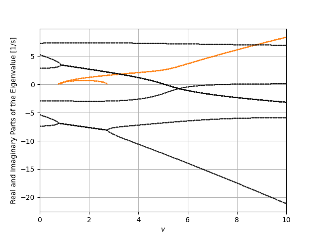
The eigenvalue parts plotted against speed \(v\) show that the model is always unstable due to the inverted pendulum eigenmode of the upper body. But the classic weave, capsize, and caster modes are visible and look similar to the rigid rider model.

vs = np.linspace(0.0, 10.0, num=401)
ax = model.plot_eigenvalue_parts(hide_zeros=True, sort_modes=False, v=vs)

If the stiffness of the rider lean joint \(k_9\) is increased, the dynamics should approach that of the rigid rider model and the self-stability can be brought back. Zoom in to see the where the model becomes stable.

k9s = np.linspace(0.0, 300.0, num=301)
ax = model.plot_eigenvalue_parts(hide_zeros=True, sort_modes=False, v=5.5,
                                 k9=k9s, c9=50.0)
ax.set_ylim((-5.0, 5.0))

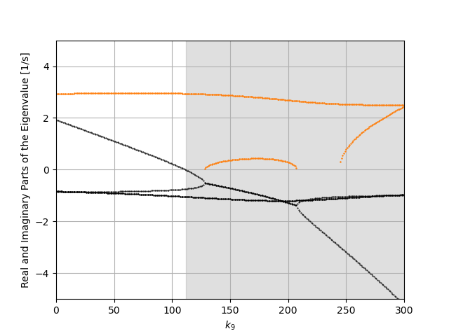
(-5.0, 5.0)

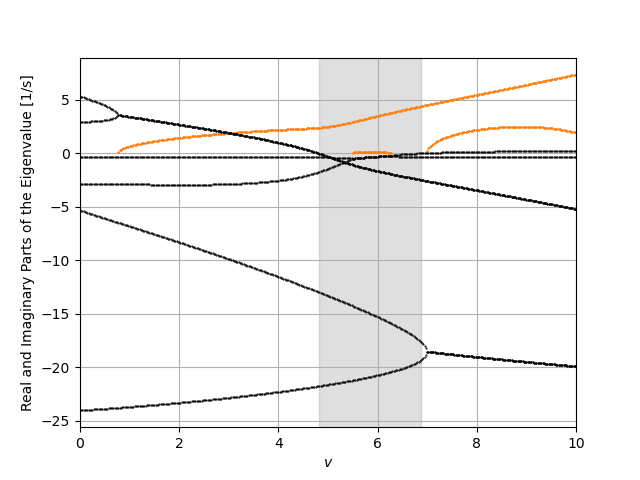
Selecting values for the passive stiffness and damping at the rider upper body joint gives dynamics with a small stable speed range.

ax = model.plot_eigenvalue_parts(hide_zeros=True, sort_modes=False, v=vs,
                                 k9=128.0, c9=50.0)

Modes of Motion

When populated with realistic parameter values the linear Carvallo-Whipple model exhibits four characteristic eigenmodes that transition into three eigenmodes when two roots bifurcate into an imaginary pair. The rider lean degree of freedom adds two real modes at low speed and an additional oscillatory mode at high speed.

Low Speed, Unstable Inverted Pendulum

ax = model.plot_eigenvectors(hide_zeros=True, v=0.0, k9=128.0, c9=50.0)

times = np.linspace(0.0, 1.0)
ax = model.plot_mode_simulations(times, hide_zeros=True, v=0.0, k9=128.0,
                                 c9=50.0)

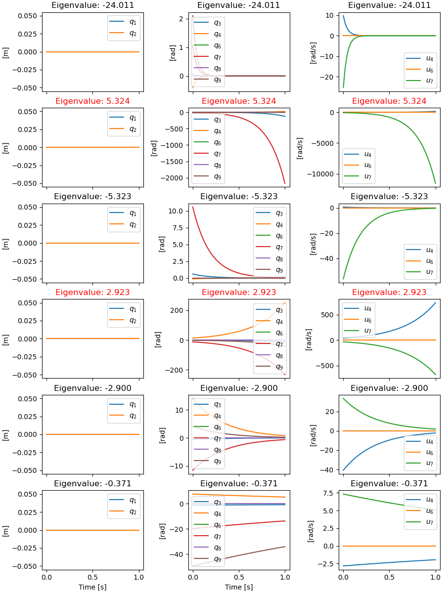
The total motion shows that the bicycle falls over.

x0 = np.zeros(12)
x0[3] = np.deg2rad(1.0)  # q4
ax = model.plot_simulation(times, x0, v=0.0, k9=128.0, c9=50.0)

Low Speed, Unstable Weave

ax = model.plot_eigenvectors(hide_zeros=True, v=2.0, k9=128.0, c9=50.0)

times = np.linspace(0.0, 1.0)
ax = model.plot_mode_simulations(times, hide_zeros=True, v=2.0, k9=128.0,
                                 c9=50.0)

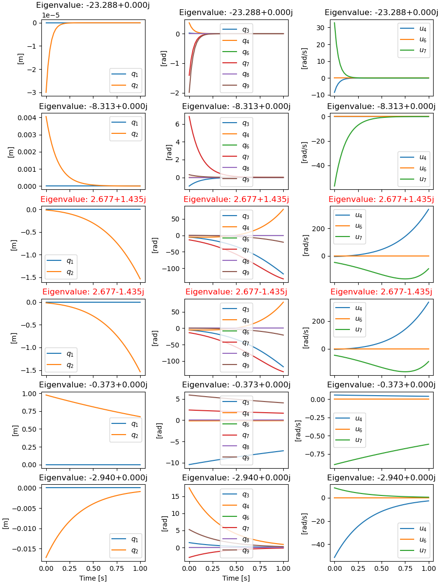
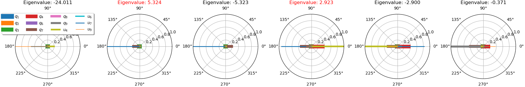
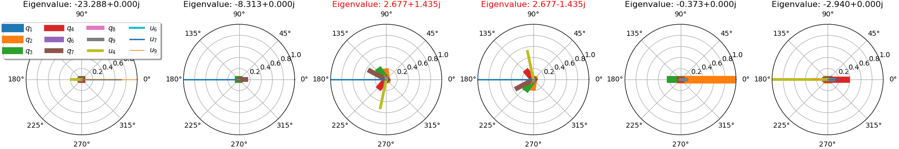
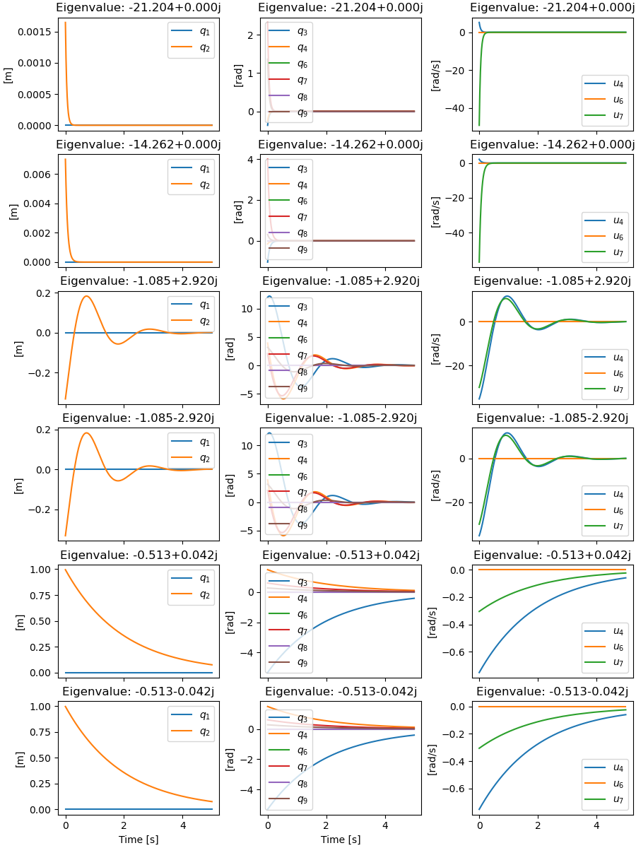
Stable Eigenmodes

ax = model.plot_eigenvectors(hide_zeros=True, v=5.5, k9=128.0, c9=50.0)

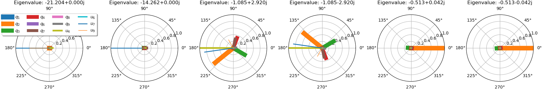
times = np.linspace(0.0, 5.0, num=501)
ax = model.plot_mode_simulations(times, hide_zeros=True, v=5.5, k9=128.0,
                                 c9=50.0)

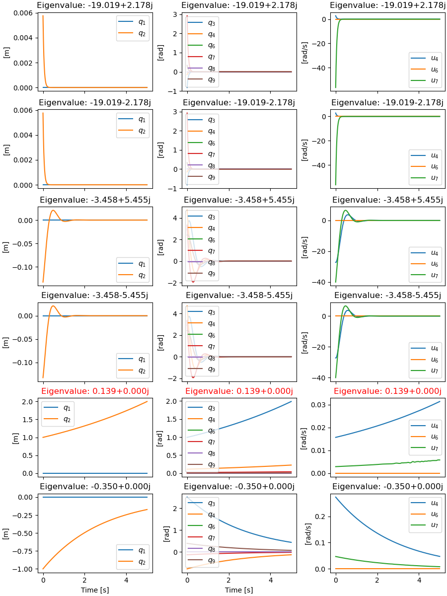
High Speed, Unstable Capsize

ax = model.plot_eigenvectors(hide_zeros=True, v=8.0, k9=128.0, c9=50.0)

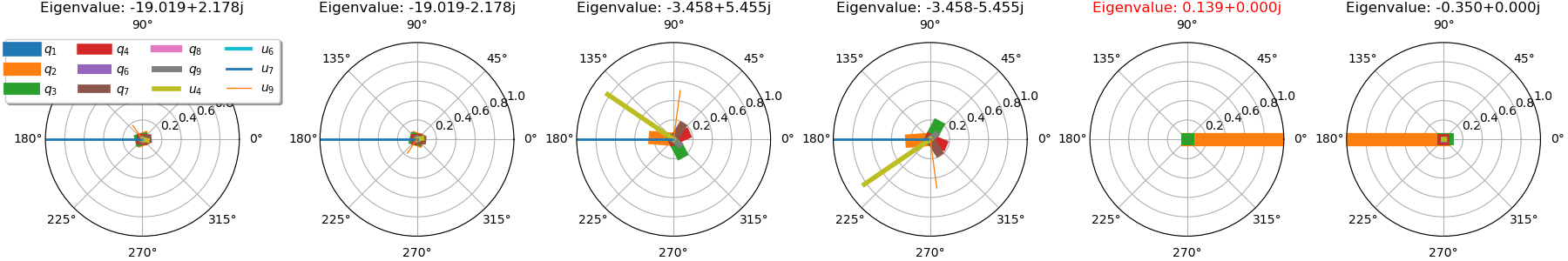
ax = model.plot_mode_simulations(times, hide_zeros=True, v=8.0, k9=128.0,
                                 c9=50.0)

Total Motion Simulation

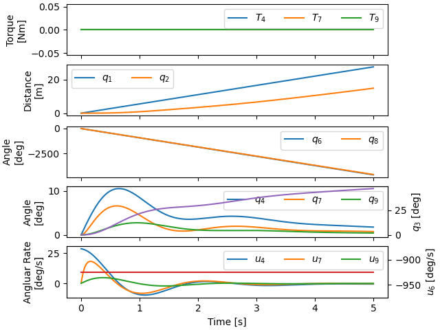
The following plot shows the total motion with an initially perturbed roll rate at 5.5 m/s.

x0 = np.zeros(12)
x0[8] = 0.5  # u4
ax = model.plot_simulation(times, x0, v=5.5, k9=128.0, c9=50.0)

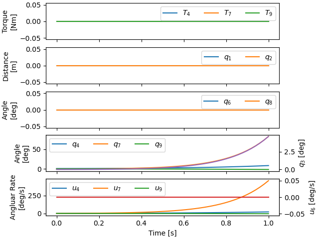
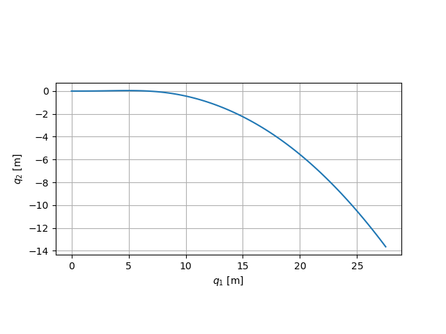
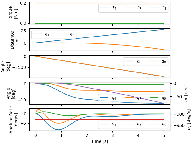
A constant steer torque puts the model into a turn, showing the step response.

times = np.linspace(0.0, 5.0, num=101)
x0 = np.zeros(12)
res, inputs = model.simulate(times, x0,
                             input_func=lambda t, x: [0.0, 0.2, 0.0],
                             v=5.5, k9=128.0, c9=50.0)
fig, ax = plt.subplots()
ax.plot(res[:, 0], res[:, 1])
ax.set_xlabel('$q_1$ [m]')
ax.set_ylabel('$q_2$ [m]')
ax.set_aspect('equal')
ax.grid()

ax = model.plot_simulation(times, x0,
                           input_func=lambda t, x: [0.0, 0.2, 0.0],
                           v=5.5, k9=128.0, c9=50.0)