Full State Feedback Control With LQR

We have a Meijaard2007WithFeedbackModel that applies full state feedback to the Meijaard2007Model using eight feedback gains. These feedback gains can be chosen with a variety of methods to stabilize the system. This example shows how to apply LQR control.

import numpy as np
from scipy.linalg import solve_continuous_are

from bicycleparameters.models import Meijaard2007WithFeedbackModel
from bicycleparameters.parameter_sets import Meijaard2007ParameterSet

Create the model and plot the eigenvalues versus speed. This should be identical to the model without feedback given that the gains are all set to zero.

par = {
    'IBxx': 11.3557360401,
    'IBxz': -1.96756380745,
    'IByy': 12.2177848012,
    'IBzz': 3.12354397008,
    'IFxx': 0.0904106601579,
    'IFyy': 0.149389340425,
    'IHxx': 0.253379594731,
    'IHxz': -0.0720452391817,
    'IHyy': 0.246138810935,
    'IHzz': 0.0955770796289,
    'IRxx': 0.0883819364527,
    'IRyy': 0.152467620286,
    'c': 0.0685808540382,
    'g': 9.81,
    'lam': 0.399680398707,
    'mB': 81.86,
    'mF': 2.02,
    'mH': 3.22,
    'mR': 3.11,
    'rF': 0.34352982332,
    'rR': 0.340958858855,
    'v': 1.0,
    'w': 1.121,
    'xB': 0.289099434117,
    'xH': 0.866949640247,
    'zB': -1.04029228321,
    'zH': -0.748236400835,
}
par_set = Meijaard2007ParameterSet(par, True)
model = Meijaard2007WithFeedbackModel(par_set)

speeds = np.linspace(0.0, 10.0, num=1001)
ax = model.plot_eigenvalue_parts(v=speeds,
                                 colors=['C0', 'C0', 'C1', 'C2'],
                                 hide_zeros=True)
ax.set_ylim((-10.0, 10.0))

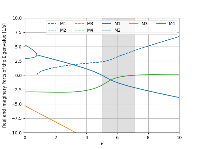
(-10.0, 10.0)

It is well known that a simple proportional positive feedback of roll angular rate to control steer torque can stabilize a bicycle at lower speeds. So set the \(k_{T_{\delta}\dot{\phi}}\) to a larger negative value.

ax = model.plot_eigenvalue_parts(v=speeds,
                                 kTdel_phid=-50.0,
                                 colors=['C0', 'C0', 'C1', 'C1'],
                                 hide_zeros=True)
ax.set_ylim((-10.0, 10.0))

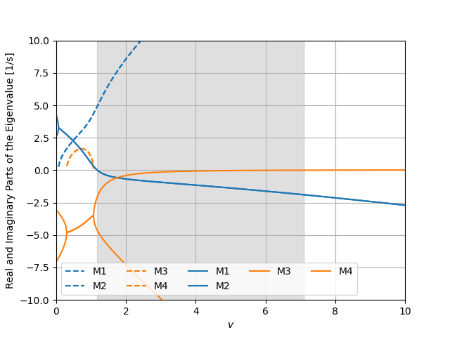
(-10.0, 10.0)

The stable speed range is significantly increased, but the weave mode eigenfrequency is increased as a consequence.

This can also be used to model adding springy training wheels by including a negative feedback of roll angle to roll torque with damping.

ax = model.plot_eigenvalue_parts(v=speeds,
                                 kTphi_phi=3000.0,
                                 kTphi_phid=600.0,
                                 hide_zeros=True)
ax.set_ylim((-10.0, 10.0))

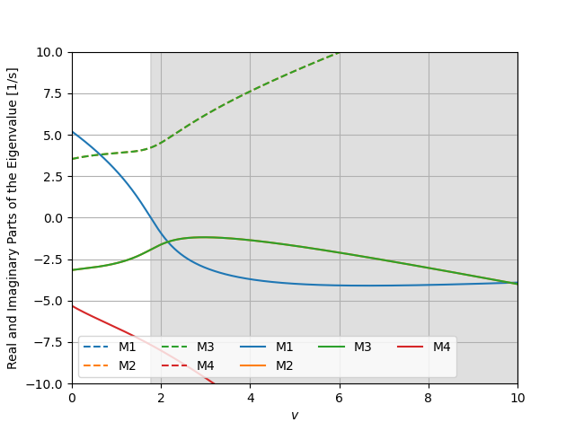
(-10.0, 10.0)

times = np.linspace(0.0, 5.0, num=1001)
model.plot_mode_simulations(times, v=2.0, kTphi_phi=3000.0,
                            kTphi_phid=600.0)

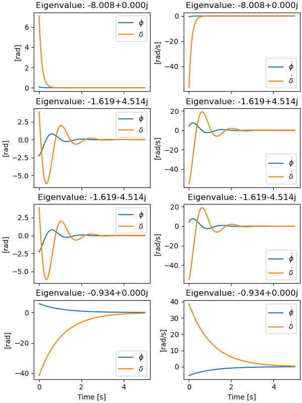
array([[<Axes: title={'center': 'Eigenvalue: -8.008+0.000j'}, ylabel='[rad]'>,
        <Axes: title={'center': 'Eigenvalue: -8.008+0.000j'}, ylabel='[rad/s]'>],
       [<Axes: title={'center': 'Eigenvalue: -1.619+4.514j'}, ylabel='[rad]'>,
        <Axes: title={'center': 'Eigenvalue: -1.619+4.514j'}, ylabel='[rad/s]'>],
       [<Axes: title={'center': 'Eigenvalue: -1.619-4.514j'}, ylabel='[rad]'>,
        <Axes: title={'center': 'Eigenvalue: -1.619-4.514j'}, ylabel='[rad/s]'>],
       [<Axes: title={'center': 'Eigenvalue: -0.934+0.000j'}, xlabel='Time [s]', ylabel='[rad]'>,
        <Axes: title={'center': 'Eigenvalue: -0.934+0.000j'}, xlabel='Time [s]', ylabel='[rad/s]'>]],
      dtype=object)

A more general method to control the bicycle is to create gain scheduling with continuous Ricatti equation. If the system is controllable, this guarantees a respect to speed using LQR optimal control. Assuming we only control steer so we will only apply control at speeds greater than 0.8 m/s. stable closed loop system. There is an uncontrollable speed just below 0.8 m/s, torque via feedback of all four states, the 4 gains can be found by solving the

As, Bs = model.form_state_space_matrices(v=speeds)
Ks = np.zeros((len(speeds), 2, 4))
Q = np.eye(4)
R = np.eye(1)

for i, (vi, Ai, Bi) in enumerate(zip(speeds, As, Bs)):
    if vi >= 0.8:
        S = solve_continuous_are(Ai, Bi[:, 1:2], Q, R)
        Ks[i, 1, :] = (np.linalg.inv(R) @ Bi[:, 1:2].T @  S).squeeze()

ax = model.plot_gains(v=speeds,
                      kTphi_phi=Ks[:, 0, 0],
                      kTphi_del=Ks[:, 0, 1],
                      kTphi_phid=Ks[:, 0, 2],
                      kTphi_deld=Ks[:, 0, 3],
                      kTdel_phi=Ks[:, 1, 0],
                      kTdel_del=Ks[:, 1, 1],
                      kTdel_phid=Ks[:, 1, 2],
                      kTdel_deld=Ks[:, 1, 3])

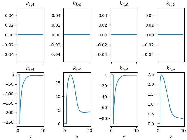
Now use the computed gains to check for closed loop stability:

ax = model.plot_eigenvalue_parts(v=speeds,
                                 kTphi_phi=Ks[:, 0, 0],
                                 kTphi_del=Ks[:, 0, 1],
                                 kTphi_phid=Ks[:, 0, 2],
                                 kTphi_deld=Ks[:, 0, 3],
                                 kTdel_phi=Ks[:, 1, 0],
                                 kTdel_del=Ks[:, 1, 1],
                                 kTdel_phid=Ks[:, 1, 2],
                                 kTdel_deld=Ks[:, 1, 3])
ax.set_ylim((-10.0, 10.0))

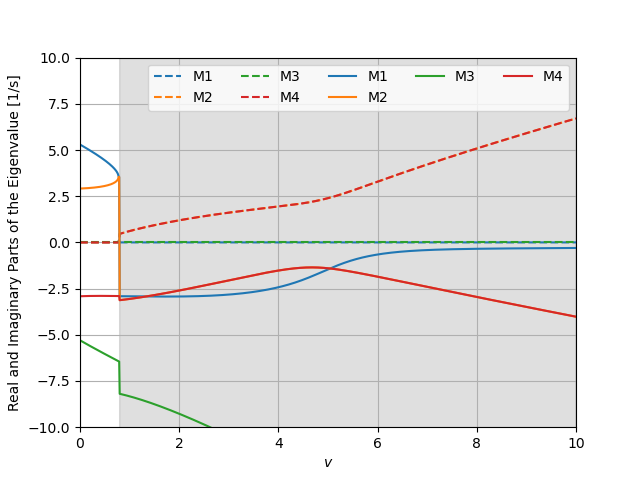
(-10.0, 10.0)

This is stable over a wide speed range and retains the weave eigenfrequency of the uncontrolled system.

x0 = np.deg2rad([5.0, -3.0, 0.0, 0.0])


def input_func(t, x):
    if (t > 2.5 and t < 2.8):
        return np.array([50.0, 0.0])
    else:
        return np.zeros(2)


times = np.linspace(0.0, 5.0, num=1001)

idx = 90
ax = model.plot_simulation(
    times,
    x0,
    input_func=input_func,
    v=speeds[idx],
    kTphi_phi=Ks[idx, 0, 0],
    kTphi_del=Ks[idx, 0, 1],
    kTphi_phid=Ks[idx, 0, 2],
    kTphi_deld=Ks[idx, 0, 3],
    kTdel_phi=Ks[idx, 1, 0],
    kTdel_del=Ks[idx, 1, 1],
    kTdel_phid=Ks[idx, 1, 2],
    kTdel_deld=Ks[idx, 1, 3],
)
ax[0].set_title('$v$ = {} m/s'.format(speeds[idx]))

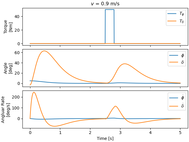
Text(0.5, 1.0, '$v$ = 0.9 m/s')