Balance Assist E-Bike with Roll Rate Feedback Steer Control

This example shows how to work with a model that includes a feedback controller and how to use a simple derivative control with it. The TU Delft Bicycle Lab developed a bicycle with a steer motor that can be controlled based on sensor measurements from an inertial measurement unit mounted on the rear frame, a steer angle sensor, and a speed sensor. The bicycle is based on an e-bike model from Royal Dutch Gazelle:

Gazelle Grenoble/Arroyo E-Bike modified with a steering motor. Battery in the downtube and electronics box on the rear rack.

import numpy as np

from bicycleparameters.main import Bicycle
from bicycleparameters.io import remove_uncertainties
from bicycleparameters.parameter_sets import Meijaard2007ParameterSet
from bicycleparameters.models import Meijaard2007WithFeedbackModel

Set Up a Model

First, load the physical parameter measurements of the bicycle from a file and create a Meijaard2007ParameterSet.

data_dir = "../../data"

bicycle = Bicycle("Balanceassistv1", pathToData=data_dir)
par = remove_uncertainties(bicycle.parameters['Benchmark'])
par['v'] = 1.0
par_set = Meijaard2007ParameterSet(par, False)
par_set

Found the RawData directory: ../../data/bicycles/Balanceassistv1/RawData
Looks like you've already got some parameters for Balanceassistv1, use forceRawCalc to recalculate.

Meijaard2007

Variable	Value
\(I_{Bxx}\)	1.120
\(I_{Bxz}\)	0.047
\(I_{Byy}\)	3.160
\(I_{Bzz}\)	2.119
\(I_{Fxx}\)	0.100
\(I_{Fyy}\)	0.190
\(I_{Hxx}\)	0.298
\(I_{Hxz}\)	-0.038
\(I_{Hyy}\)	0.257
\(I_{Hzz}\)	0.057
\(I_{Rxx}\)	0.102
\(I_{Ryy}\)	0.189
\(c\)	0.042
\(g\)	9.807
\(\lambda\)	0.255
\(m_B\)	22.500
\(m_F\)	2.235
\(m_H\)	4.300
\(m_R\)	4.085
\(r_F\)	0.352
\(r_R\)	0.349
\(v\)	1.000
\(w\)	1.113
\(x_B\)	0.519
\(x_H\)	0.921
\(z_B\)	-0.521
\(z_H\)	-0.860

The following plot depicts the geometry and inertial parameters with the inertia of the rider included.

par_set.plot_all()

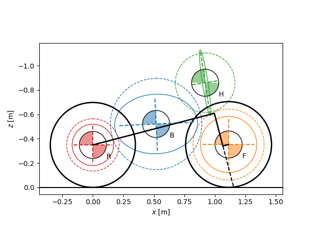
<Axes: xlabel='$x$ [m]', ylabel='$z$ [m]'>

Create a Meijaard2007WithFeedbackModel. The parameter set does not include the feedback gain parameters, but to_parameterization() will be used to convert the parameter set into one with the gains.

model = Meijaard2007WithFeedbackModel(par_set)
model.parameter_set

Meijaard2007WithFeedback

Variable	Value
\(I_{Bxx}\)	1.120
\(I_{Bxz}\)	0.047
\(I_{Byy}\)	3.160
\(I_{Bzz}\)	2.119
\(I_{Fxx}\)	0.100
\(I_{Fyy}\)	0.190
\(I_{Hxx}\)	0.298
\(I_{Hxz}\)	-0.038
\(I_{Hyy}\)	0.257
\(I_{Hzz}\)	0.057
\(I_{Rxx}\)	0.102
\(I_{Ryy}\)	0.189
\(c\)	0.042
\(g\)	9.807
\(k_{T_{\delta}\delta}\)	0.000
\(k_{T_{\delta}\dot{\delta}}\)	0.000
\(k_{T_{\delta}\phi}\)	0.000
\(k_{T_{\delta}\dot{\phi}}\)	0.000
\(k_{T_{\phi}\delta}\)	0.000
\(k_{T_{\phi}\dot{\delta}}\)	0.000
\(k_{T_{\phi}\phi}\)	0.000
\(k_{T_{\phi}\dot{\phi}}\)	0.000
\(\lambda\)	0.255
\(m_B\)	22.500
\(m_F\)	2.235
\(m_H\)	4.300
\(m_R\)	4.085
\(r_F\)	0.352
\(r_R\)	0.349
\(v\)	1.000
\(w\)	1.113
\(x_B\)	0.519
\(x_H\)	0.921
\(z_B\)	-0.521
\(z_H\)	-0.860

The model shows a small self-stable speed range.

speeds = np.linspace(0.0, 10.0, num=501)
ax = model.plot_eigenvalue_parts(v=speeds)
ax.set_ylim((-10.0, 10.0))

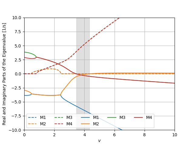
(-10.0, 10.0)

Add a Rider

If the data files for a rider are present in the data directory, you can add a rider and the package Yeadon will be used to configure a rider to sit on the bicycle. You can check if a rider is properly configured by plotting the geometry which will now include a stick figure depiction of the rider.

bicycle.add_rider('Jason', reCalc=True)
bicycle.plot_bicycle_geometry(inertiaEllipse=False)

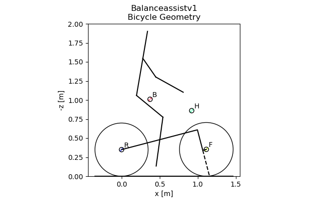
There is no rider on the bicycle, now adding Jason.
Calculating the human configuration.

<Figure size 647.214x400 with 1 Axes>

The inertia representation now reflects the larger inertia of the rear frame due to the rigid rider addition.

par = remove_uncertainties(bicycle.parameters['Benchmark'])
par['v'] = 1.0
par_set = Meijaard2007ParameterSet(par, True)
par_set.plot_all()

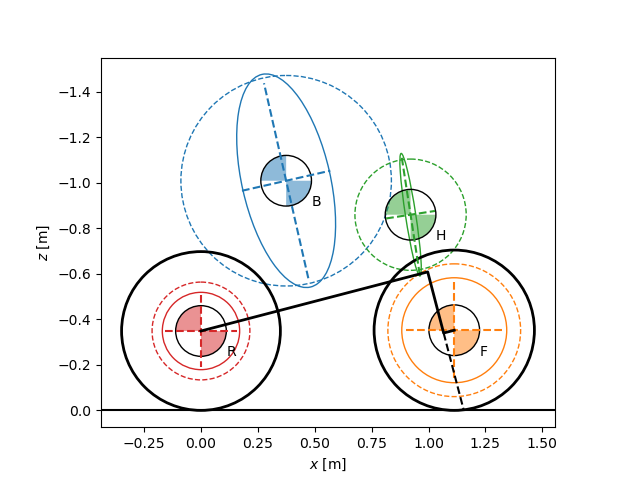
<Axes: xlabel='$x$ [m]', ylabel='$z$ [m]'>

The self-stable speed range begins at a higher speed and becomes wider.

model = Meijaard2007WithFeedbackModel(par_set)
ax = model.plot_eigenvalue_parts(v=speeds)
ax.set_ylim((-10.0, 10.0))

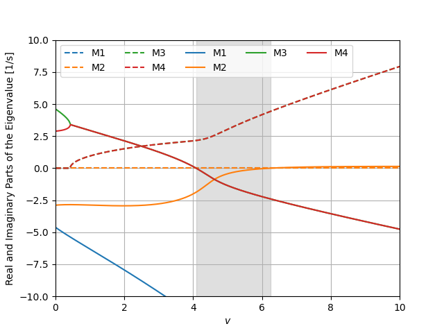
(-10.0, 10.0)

Add Control

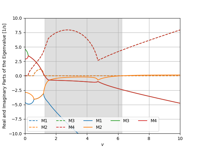
It turns out that controlling the steer torque with a positive feedback on roll angular rate, the bicycle can be stabilized over a large speed range. For example, setting \(k_{T_\delta \dot{\phi}}=-50\) gives this effect:

ax = model.plot_eigenvalue_parts(v=speeds, kTdel_phid=-50.0)
ax.set_ylim((-10.0, 10.0))

(-10.0, 10.0)

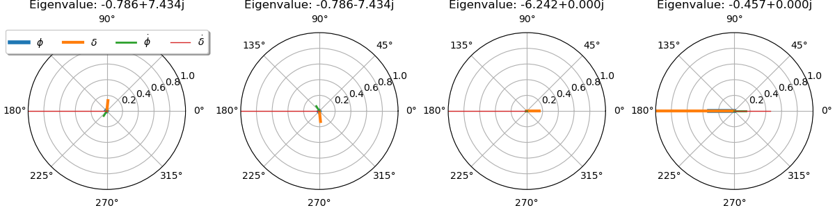
The eigenvectors at low speed show that the weave mode has a steer dominated high frequency natural motion. This may not be so favorable.

speed = 2.0
ax = model.plot_eigenvectors(v=speed, kTdel_phid=-50.0)

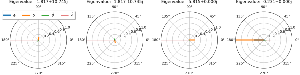
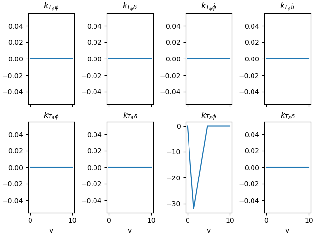
You can also gain schedule with respect to speed. A linear variation in the roll rate gain can make the weave eigenfrequency have lower magnitude than using simply a constant gain.

vmin, vmin_idx = 1.5, np.argmin(np.abs(speeds - 1.5))
vmax, vmax_idx = 4.7, np.argmin(np.abs(speeds - 4.7))
kappa = 10.0
kphidots = -kappa*(vmax - speeds)
kphidots[:vmin_idx] = -kappa*(vmax - vmin)/vmin*speeds[:vmin_idx]
kphidots[vmax_idx:] = 0.0
model.plot_gains(v=speeds, kTdel_phid=kphidots)

array([[<Axes: title={'center': '$k_{T_{\\phi}\\phi}$'}>,
        <Axes: title={'center': '$k_{T_{\\phi}\\delta}$'}>,
        <Axes: title={'center': '$k_{T_{\\phi}\\dot{\\phi}}$'}>,
        <Axes: title={'center': '$k_{T_{\\phi}\\dot{\\delta}}$'}>],
       [<Axes: title={'center': '$k_{T_{\\delta}\\phi}$'}, xlabel='v'>,
        <Axes: title={'center': '$k_{T_{\\delta}\\delta}$'}, xlabel='v'>,
        <Axes: title={'center': '$k_{T_{\\delta}\\dot{\\phi}}$'}, xlabel='v'>,
        <Axes: title={'center': '$k_{T_{\\delta}\\dot{\\delta}}$'}, xlabel='v'>]],
      dtype=object)

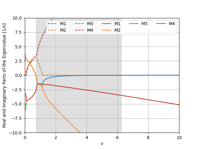
Using the gain scheduling gives this effect to the dynamics:

ax = model.plot_eigenvalue_parts(v=speeds, kTdel_phid=kphidots)
ax.set_ylim((-10.0, 10.0))

(-10.0, 10.0)

kphidot = kphidots[np.argmin(np.abs(speeds - speed))]
ax = model.plot_eigenvectors(v=speed, kTdel_phid=kphidot)

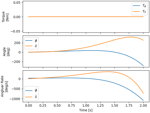
We can then simulate the system at a specific low speed and see the effect control has. First, without control:

times = np.linspace(0.0, 2.0, num=201)
x0 = np.array([0.0, 0.0, 0.5, 0.0])
ax = model.plot_simulation(times, x0, v=speed)

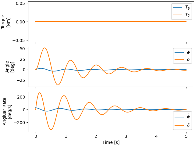
And with control:

times = np.linspace(0.0, 5.0, num=501)
ax = model.plot_simulation(times, x0, v=speed, kTdel_phid=kphidot)