Benchmark Carvallo-Whipple Model

Meijaard et al. presents a benchmark minimal linear Carvallo-Whipple bicycle model ([Meijaard2007], [Carvallo1899], [Whipple1899]) with 27 unique constant parameters and two coordinates: roll angle \(\phi\) and steer angle \(\delta\).

import numpy as np

from bicycleparameters import Bicycle
from bicycleparameters.io import remove_uncertainties
from bicycleparameters.parameter_sets import Meijaard2007ParameterSet
from bicycleparameters.models import Meijaard2007Model

data_dir = "../../data"

Benchmark Parameter Values

First, create a Bicycle object from the parameter file in the data directory.

bicycle = Bicycle("Benchmark", pathToData=data_dir)

Looks like you've already got some parameters for Benchmark, use forceRawCalc to recalculate.

Strip the uncertainties from the parameters and add a speed parameter \(v\), then create a Meijaard2007ParameterSet set from the parameter values.

par = remove_uncertainties(bicycle.parameters['Benchmark'])
par['v'] = 4.6
par_set = Meijaard2007ParameterSet(par, True)
par_set

Meijaard2007

Variable	Value
\(I_{Bxx}\)	9.200
\(I_{Bxz}\)	2.400
\(I_{Byy}\)	11.000
\(I_{Bzz}\)	2.800
\(I_{Fxx}\)	0.141
\(I_{Fyy}\)	0.280
\(I_{Hxx}\)	0.059
\(I_{Hxz}\)	-0.008
\(I_{Hyy}\)	0.060
\(I_{Hzz}\)	0.007
\(I_{Rxx}\)	0.060
\(I_{Ryy}\)	0.120
\(c\)	0.080
\(g\)	9.810
\(\lambda\)	0.314
\(m_B\)	85.000
\(m_F\)	3.000
\(m_H\)	4.000
\(m_R\)	2.000
\(r_F\)	0.350
\(r_R\)	0.300
\(v\)	4.600
\(w\)	1.020
\(x_B\)	0.300
\(x_H\)	0.900
\(z_B\)	-0.900
\(z_H\)	-0.700

The bicycle geometry and representations of the inertia of the four rigid bodies (B: rear frame, F: front wheel, H: front frame, R: rear wheel) can be visualized with the parameter set plot methods.

ax = par_set.plot_all()

Linear Carvallo-Whipple Model

Create a Meijaard2007Model that represents linear Carvallo-Whipple model presented in [Meijaard2007] and populate it with the parameter values in the parameter set.

model = Meijaard2007Model(par_set)

This model can be written in this form:

\[\mathbf{M}\ddot{\vec{q}} + v\mathbf{C}_1\dot{\vec{q}} + \left[ g \mathbf{K}_0 + v^2 \mathbf{K}_2 \right] \vec{q} = \vec{F}\]

where the essential coordinates are the roll angle \(\phi\) and steer angle \(\delta\), respectively:

\[\vec{q} = [\phi \quad \delta]^T\]

and the forcing terms are:

\[\vec{F} = [T_\phi \quad T_\delta]^T\]

The model can calculate the mass, damping, and stiffness coefficient matrices, which should match the paper’s results when using the matching parameter values:

M, C1, K0, K2 = model.form_reduced_canonical_matrices()
M

array([[80.817,  2.319],
       [ 2.319,  0.298]])

C1

array([[ 0.   , 33.866],
       [-0.85 ,  1.685]])

K0

array([[-80.95 ,  -2.6  ],
       [ -2.6  ,  -0.803]])

K2

array([[ 0.   , 76.597],
       [ 0.   ,  2.654]])

The root locus can be plotted as a function of any model parameter. This plot is most often used to show how stability is dependent on the speed parameter.The blue lines indicate the weave eigenmode, the green the capsize eigenmode, and the orange the caster eigenmode. Vertical dashed lines indicate speeds that are examined further below.

v = np.linspace(0.0, 10.0, num=401)
ax = model.plot_eigenvalue_parts(v=v,
                                 colors=['C0', 'C0', 'C1', 'C2'],
                                 hide_zeros=True)
for vi in [0.0, 2.0, 5.0, 8.0]:
    ax.axvline(vi, color='k', linestyle='--')
ax.set_ylim((-10.0, 10.0))

(-10.0, 10.0)

Modes of Motion

When populated with realistic parameter values the linear Carvallo-Whipple model exhibits four characteristic eigenmodes that transition into three eigenmodes when two roots bifurcate into an imaginary pair.

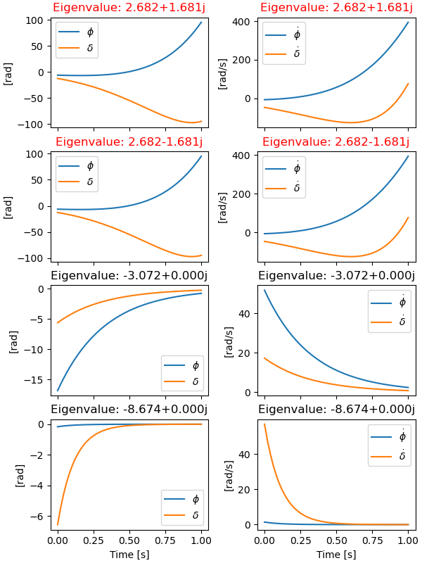
Low Speed, Unstable Inverted Pendulum

Before the bifurcation point into the weave mode, there are four real eigenvalues that describe the motion.

ax = model.plot_eigenvectors(v=0.0)

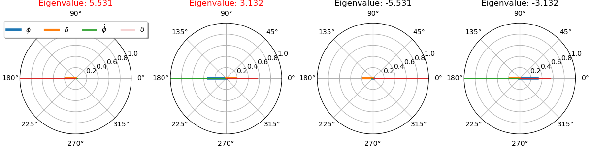
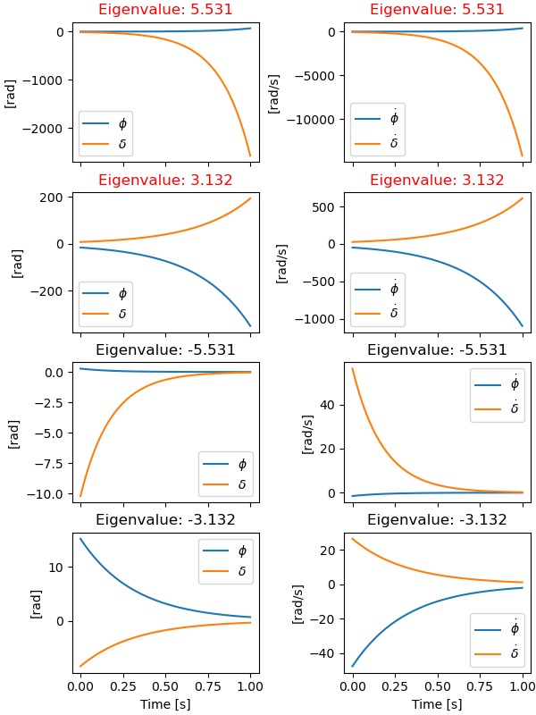
The unstable eigenmodes dominate the motion and this results in the steer angle growing rapidly and the roll angle following suite, but slower.

times = np.linspace(0.0, 1.0)
ax = model.plot_mode_simulations(times, v=0.0)

The total motion shows that the bicycle falls over, as expected.

ax = model.plot_simulation(times, [0.01, 0.0, 0.0, 0.0], v=0.0)

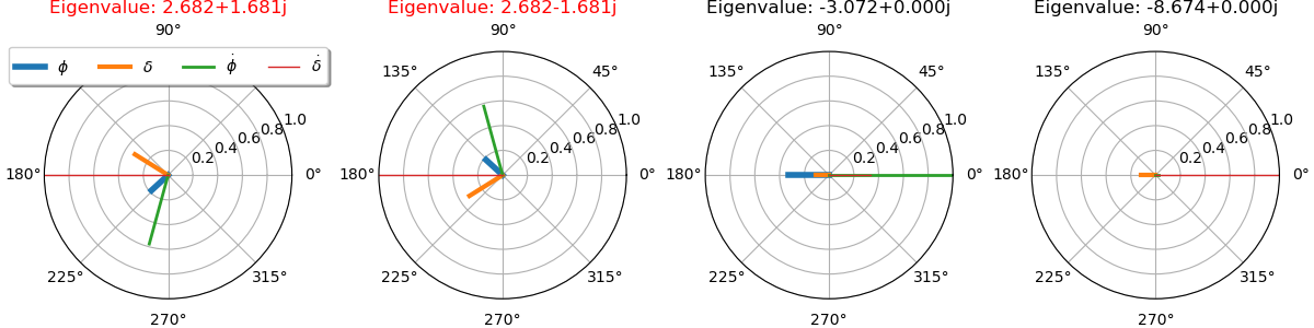
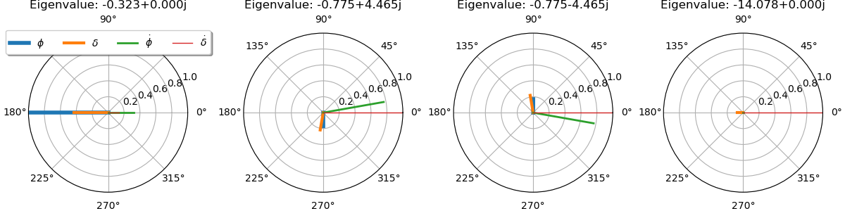
Low Speed, Unstable Weave

Moving up in speed past the bifurcation, the bicycle has an unstable oscillatory eigenmode that is called “weave”. The steer angle has about twice the magnitude as the roll angle and they both grow together with close to 90 degrees phase. The other two stable real valued eigenmodes are called “capsize” and “caster”, with capsize being primarily a roll motion and caster a steer motion.

ax = model.plot_eigenvectors(v=2.0)

times = np.linspace(0.0, 1.0)
ax = model.plot_mode_simulations(times, v=2.0)

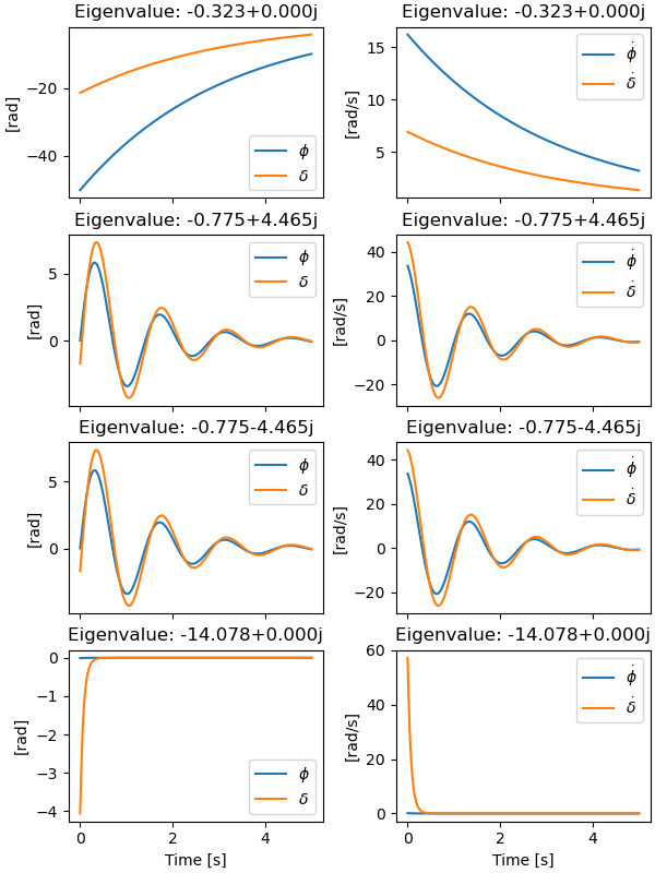
Stable Eigenmodes

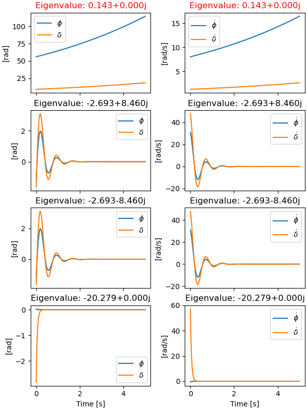
Increasing speed further shows that the weave eigenmode becomes stable, making all eigenmodes stable, and thus the total motion is stable. The speed regime where this is true is called the “self-stable” speed range given that stability arises with no active control. The weave steer-roll phase is almost aligned and the caster time constant is becoming very fast.

ax = model.plot_eigenvectors(v=5.0)

times = np.linspace(0.0, 5.0, num=501)
ax = model.plot_mode_simulations(times, v=5.0)

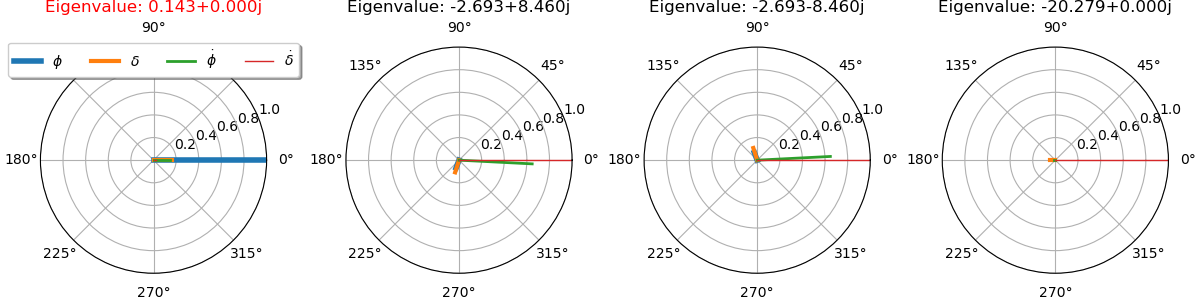
High Speed, Unstable Capsize

If the speed is increased further, the system becomes unstable due to the capsize mode. The weave steer and roll are mostly aligned in phase but the roll dominated capsize shows that the bicycle slowly falls over.

ax = model.plot_eigenvectors(v=8.0)

ax = model.plot_mode_simulations(times, v=8.0)

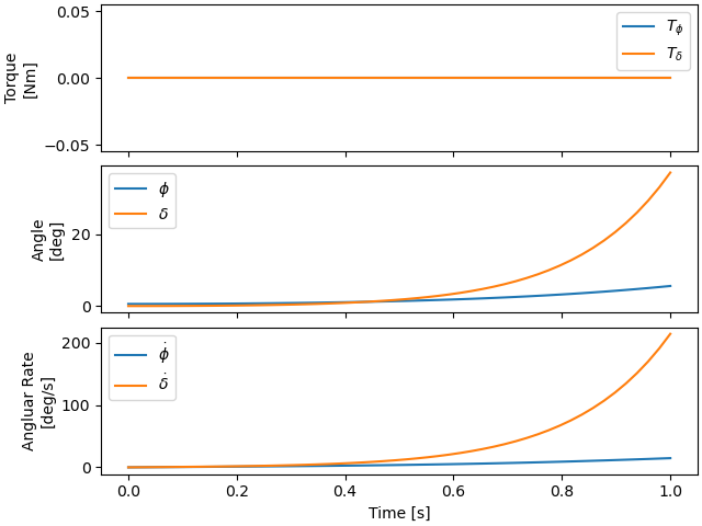
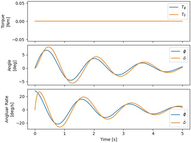
Total Motion Simulation

The following plot shows the total motion with the same initial conditions used in [Meijaard2007] within the stable speed range at 4.6 m/s.

x0 = [0.0, 0.0, 0.5, 0.0]
ax = model.plot_simulation(times, x0)

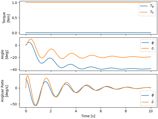
A constant steer torque puts the model into a turn.

times = np.linspace(0.0, 10.0, num=1001)
ax = model.plot_simulation(times, x0,
                           input_func=lambda t, x: [0.0, 1.0])