Using Models

Parameter sets can be associated with a model and the model can be used to compute and visualize properties of the model’s dynamics.

import numpy as np
from bicycleparameters.parameter_dicts import meijaard2007_browser_jason
from bicycleparameters.parameter_sets import Meijaard2007ParameterSet
from bicycleparameters.models import Meijaard2007Model

np.set_printoptions(precision=3, suppress=True)

Start with a parameter and construct a model with it:

par_set = Meijaard2007ParameterSet(meijaard2007_browser_jason, True)
model = Meijaard2007Model(par_set)

Model Attributes

Models have a set of ordered state variables:

model.state_vars

['phi', 'delta', 'phidot', 'deltadot']

model.state_units

['rad', 'rad', 'rad/s', 'rad/s']

model.state_vars_latex

['\\phi', '\\delta', '\\dot{\\phi}', '\\dot{\\delta}']

Models have a set of ordered input variables:

model.input_vars

['Tphi', 'Tdelta']

model.input_units

['N-m', 'N-m']

model.input_vars_latex

['T_\\phi', 'T_\\delta']

State Space

All linear models have a method that generates the state and input matrices. The rows and columns match the order of the state and input variables.

A, B = model.form_state_space_matrices()
A

array([[ 0.   ,  0.   ,  1.   ,  0.   ],
       [ 0.   ,  0.   ,  0.   ,  1.   ],
       [ 8.262, -0.947, -0.03 , -0.214],
       [17.665, 26.246,  1.993, -2.844]])

B

array([[ 0.   ,  0.   ],
       [ 0.   ,  0.   ],
       [ 0.011, -0.066],
       [-0.066,  4.426]])

Most all methods on models accept override values for the parameters. So if you want the state and input matrices with \(v=14,g=5.1\) and \(w=2\) pass them in as keyword arguments:

A, B = model.form_state_space_matrices(v=14.0, g=5.1, w=2.0)
A

array([[  0.   ,   0.   ,   1.   ,   0.   ],
       [  0.   ,   0.   ,   0.   ,   1.   ],
       [  4.418, -79.135,   0.027,  -2.049],
       [ -1.456,  17.075,   2.721,   2.831]])

B

array([[0.   , 0.   ],
       [0.   , 0.   ],
       [0.01 , 0.005],
       [0.005, 0.454]])

Eigenmodes

All linear models can produce its eigenvalues and eigenvectors:

evals, evecs = model.calc_eigen()
evals

array([-6.744+0.j   , -2.915+0.j   ,  3.392+0.611j,  3.392-0.611j])

evecs

array([[ 0.002+0.j   , -0.295+0.j   ,  0.043-0.075j,  0.043+0.075j],
       [ 0.147+0.j   ,  0.134+0.j   , -0.261+0.047j, -0.261-0.047j],
       [-0.013+0.j   ,  0.861+0.j   ,  0.193-0.229j,  0.193+0.229j],
       [-0.989+0.j   , -0.392+0.j   , -0.913+0.j   , -0.913-0.j   ]])

Parameters can be overridden as before, but the following line shows how you can pass in an iterable of values for any parameter override and get back an iterable of eigenvalues:

evals, evecs = model.calc_eigen(v=[2.0, 5.0])
evals

array([[ -8.143+0.j   ,  -2.967+0.j   ,   2.681+1.378j,   2.681-1.378j],
       [-12.638+0.j   ,  -1.726+0.j   ,  -0.003+2.35j ,  -0.003-2.35j ]])

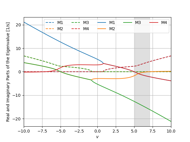
The root locus with respect to any parameter, for example here speed v, can be plotted, which uses the iterable of eigenvalues shown above:

speeds = np.linspace(-10.0, 10.0, num=200)
_ = model.plot_eigenvalue_parts(v=speeds)

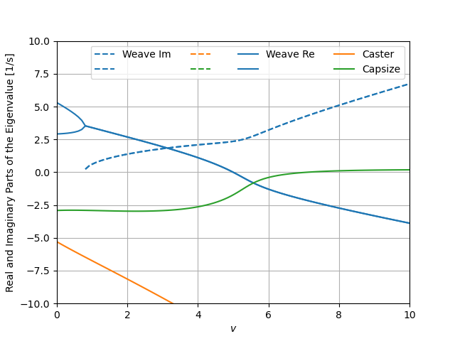
There are several common customization options available for this plot:

speeds = np.linspace(0.0, 10.0, num=100)
ax = model.plot_eigenvalue_parts(v=speeds,
                                 colors=['C0', 'C0', 'C1', 'C2'],
                                 show_stable_regions=False,
                                 hide_zeros=True)
ax.set_ylim((-10.0, 10.0))
_ = ax.legend(['Weave Im', None, None, None,
               'Weave Re', None, 'Caster', 'Capsize'], ncol=4)

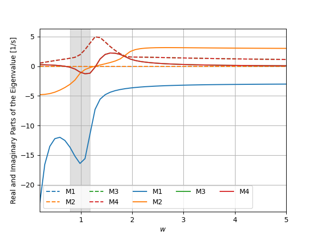
You can choose any parameter in the dictionary to generate the root locus and also override other parameters.

wheelbases = np.linspace(0.2, 5.0, num=50)
_ = model.plot_eigenvalue_parts(v=6.0, w=wheelbases)

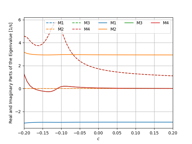
It is also possible to pass iterables for multiple parameters as long as the length is the same for all. Only the scale for the first will be shown.

trails = np.linspace(-0.2, 0.2, num=50)
wheelbases = np.linspace(0.2, 5.0, num=50)
_ = model.plot_eigenvalue_parts(c=trails, w=wheelbases)

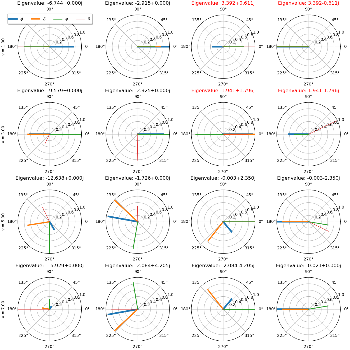
The eigenvector components can be created for each mode and for a series of parameter values:

_ = model.plot_eigenvectors(v=[1.0, 3.0, 5.0, 7.0])

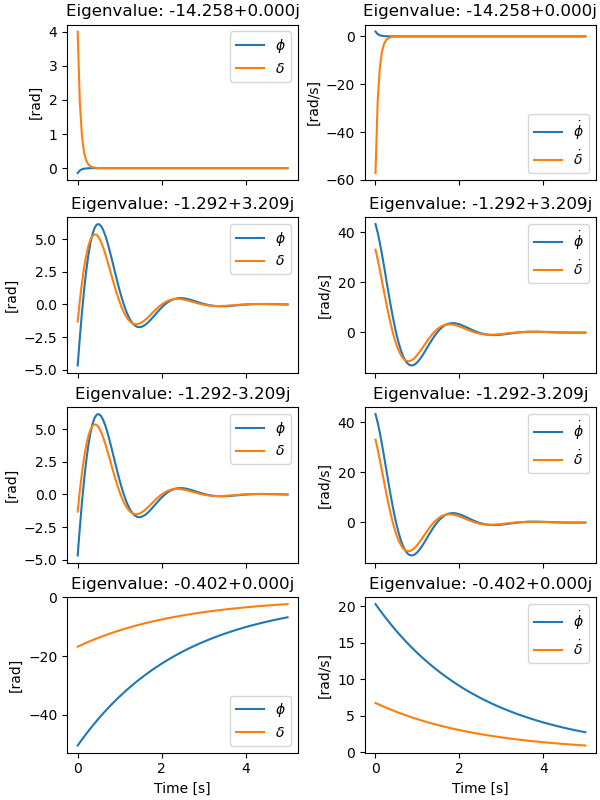
The eigenmodes can be simulated for specific parameter values:

times = np.linspace(0.0, 5.0, num=100)
_ = model.plot_mode_simulations(times, v=6.0)

Simulation

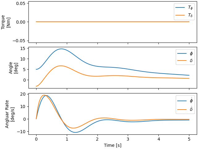
A general simulation from initial conditions can also be run:

x0 = np.deg2rad([5.0, -3.0, 0.0, 0.0])
_ = model.plot_simulation(times, x0, v=6.0)

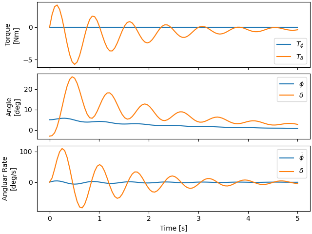
Inputs can be applied in the simulation, for example a simple positive feedback derivative controller on roll shows that the low speed bicycle can be stabilized:

x0 = np.deg2rad([5.0, -3.0, 0.0, 0.0])
_ = model.plot_simulation(times, x0,
                          input_func=lambda t, x: np.array([0.0, 50.0*x[2]]),
                          v=2.0)