Using Bicycles

import pprint
from pathlib import Path

import numpy as np
import bicycleparameters as bp
from bicycleparameters import Bicycle, tables

Loading Bicycle Data

To load the data from one of the bicycles in the data folder, instantiate a Bicycle object using the bicycle’s name:

bicycle = Bicycle('Stratos', pathToData='../data')

Found the RawData directory: ../data/bicycles/Stratos/RawData
Recalcuting the parameters.
The glory of the Stratos parameters are upon you!

This will create an instance of the Bicycle class in the variable bicycle based off of input data from the ./bicycles/Stratos/ directory. The program first looks to see if there are any parameter sets in ./bicycles/Stratos/Parameters/. If so, it loads the data, if not it looks for ./bicycles/Stratos/RawData/StratosMeasurments.txt so that it can generate the parameter set. The raw measurement file may or may not contain the oscillation period data for the bicycle moment of inertia calculations. If it doesn’t then the program will look for the series of .mat files need to calculate the periods. If no data is there, then you get an error.

There are other loading options:

bicycle = Bicycle('Stratos', pathToData='..', forceRawCalc=True,
                     forcePeriodCalc=True)

The pathToData option allows you specify a directory other than the current directory as your data directory. The forceRawCalc forces the program to load ./bicycles/Stratos/RawData/StratosMeasurments.txt and recalculate the parameters regardless if there are any parameter files available in ./bicycles/Stratos/Parameters/. The forcePeriodCalc option forces the period calculation from the .mat files regardless if they already exist in the raw measurement file.

Exploring Bicycle Parameter Data

The bicycle has a name:

bicycle.bicycleName

'Stratos'

and a directory where its data is sourced:

bicycle.directory

'../data/bicycles/Stratos'

The benchmark bicycle parameters from [Meijaard2007] are the fundamental parameter set that is used behind the scenes for calculations. To access them type:

b_par = bicycle.parameters['Benchmark']
pprint.pprint(b_par)

{'IBxx': 0.3728775783567887+/-0.0015667031268957702,
 'IBxz': -0.03834761674810283+/-0.00041198945835815804,
 'IByy': 0.7171736482966189+/-0.0031346383690536894,
 'IBzz': 0.45472945576461815+/-0.0018865067694859123,
 'IFxx': 0.09156382237275022+/-0.00037264374475717767,
 'IFyy': 0.15678445500719673+/-0.0011443558970956002,
 'IHxx': 0.17684141949871102+/-0.0008247358323528924,
 'IHxz': -0.027331980252591023+/-0.000575667418054312,
 'IHyy': 0.14362051582791002+/-0.002481616129881456,
 'IHzz': 0.044632358231408514+/-0.00030908148376534593,
 'IRxx': 0.09387109992870839+/-0.000382033804274545,
 'IRyy': 0.1542264480253569+/-0.0011387182056513865,
 'c': 0.05626998711805831+/-0.0016271109815356594,
 'g': 9.81+/-0.01,
 'lam': 0.29496064358704177+/-0.003490658503988659,
 'mB': 7.22+/-0.02,
 'mF': 3.334+/-0.02,
 'mH': 3.04+/-0.02,
 'mR': 3.96+/-0.02,
 'rF': 0.340003929196009+/-0.00012242687930145795,
 'rR': 0.338477091115578+/-0.00011368210220849667,
 'w': 1.037+/-0.002,
 'xB': 0.32631503794489763+/-0.0032538862692938647,
 'xH': 0.9106573267080197+/-0.0037388403092143935,
 'zB': -0.48263958289208314+/-0.0026376802487648857,
 'zH': -0.7302812158759062+/-0.0024284656294034685}

b_par['xB']

0.32631503794489763+/-0.0032538862692938647

The program automatically calculates the uncertainties in the parameters based on the raw measurements or the uncertainties provided in the parameter files. If you’d like to work with the pure values you can remove them from the entire dictionary:

b_par_pure = bp.io.remove_uncertainties(b_par)
b_par_pure['xB']

0.32631503794489763

or any single uncertainity quantity’s nominal value can be extracted with:

b_par['xB'].nominal_value

0.32631503794489763

That goes the same for all values with uncertainties. Check out the uncertainties package details for more ways to manipulate the quantities.

If the bicycle was calculated from raw data measurements you can access them by:

pprint.pprint(bicycle.parameters['Measured'])

{'LhbF': np.float64(0.6552),
 'LhbR': np.float64(1.1014),
 'TcB1': 1.59880197567+/-6.3096072159e-06,
 'TcF1': 1.35366619175+/-5.30396954785e-06,
 'TcH1': 1.45406634451+/-1.95301826402e-05,
 'TcR1': 1.31217723331+/-7.33295949904e-06,
 'TtB1': 1.815949139+/-1.36701497554e-05,
 'TtB2': 1.58519804957+/-9.16825068389e-06,
 'TtB3': 1.66019943538+/-8.06563293967e-06,
 'TtF1': 0.801625248455+/-1.12728802487e-06,
 'TtH1': 1.01149389309+/-4.48284908821e-06,
 'TtH2': 0.525350778277+/-2.21244434089e-06,
 'TtH3': 1.08603695606+/-5.66372430716e-06,
 'TtP1': 1.89399317145+/-5.93377589066e-06,
 'TtR1': 0.811662317594+/-9.30058972579e-07,
 'aB1': 0.249+/-0.003,
 'aB2': -0.267+/-0.003,
 'aB3': -0.071+/-0.003,
 'aH1': 0.329+/-0.003,
 'aH2': -0.038+/-0.003,
 'aH3': 0.4+/-0.003,
 'alphaB1': 128.9+/-0.2,
 'alphaB2': 221.6+/-0.2,
 'alphaB3': 184.5+/-0.2,
 'alphaH1': 36.0+/-0.2,
 'alphaH2': 94.0+/-0.2,
 'alphaH3': 347.3+/-0.2,
 'dF': 27.772+/-0.01,
 'dP': 0.03+/-0.0001,
 'dR': 29.774+/-0.01,
 'f': 0.045+/-0.001,
 'g': 9.81+/-0.01,
 'gamma': 73.1+/-0.2,
 'hbb': np.float64(0.29),
 'lF': 0.297+/-0.001,
 'lP': 1.05+/-0.001,
 'lR': 0.2965+/-0.001,
 'lamst': np.float64(1.308996939),
 'lcs': np.float64(0.445),
 'lsp': np.float64(0.195),
 'lst': np.float64(0.48),
 'mB': 7.22+/-0.02,
 'mF': 3.334+/-0.02,
 'mH': 3.04+/-0.02,
 'mP': 5.56+/-0.02,
 'mR': 3.96+/-0.02,
 'nF': np.float64(13.0),
 'nR': np.float64(14.0),
 'w': 1.037+/-0.002,
 'whb': np.float64(0.58)}

All parameter sets are stored in the parameter dictionary of the bicycle instance, which is mutable. To modify a parameter type:

bicycle.parameters['Benchmark']['mB'] = 50.0
bicycle.parameters['Benchmark']['mB']

50.0

You can regenerate the parameter sets from the raw data stored in the bicycle’s directory by calling and resetting the parameters:

par, extra = bicycle.calculate_from_measured()
bicycle.parameters['Benchmark'] = par
bicycle.parameters['Benchmark']['mB']

7.22+/-0.02

Basic Linear Model Analysis

The Bicycle object has some basic bicycle analysis tools based on the linear Carvallo-Whipple bicycle model which has been linearized about the upright configuration. For example, the canonical coefficient matrices for the equations of motion can be computed:

M, C1, K0, K2 = bicycle.canonical()
M

array([[4.8773556938672025+/-0.023934341307719046,
        0.40791147549242046+/-0.008524955893962296],
       [0.40791147549242046+/-0.008524955893962296,
        0.20324563385641692+/-0.002358205055360836]], dtype=object)

C1

array([[0.0, 4.852002528879055+/-0.024294894019445835],
       [-0.4888089303250309+/-0.0035871046725125507,
        0.7514232981989066+/-0.011819041279142298]], dtype=object)

K0

array([[-8.178655065500777+/-0.028197632940217446,
        -0.7097919259369844+/-0.013158888467975648],
       [-0.7097919259369844+/-0.013158888467975648,
        -0.20633806986820977+/-0.005713958418318107]], dtype=object)

K2

array([[0.0, 8.392121154615824+/-0.03139795630613271],
       [0.0, 0.7785916890571186+/-0.01280424781722948]], dtype=object)

as well as the state and input matrices for state space form at a particular speed, here 1.34 m/s:

A, B = bicycle.state_space(1.34)
A

array([[0.0, 0.0, 1.0, 0.0],
       [0.0, 0.0, 0.0, 1.0],
       [16.324961318973738+/-0.03920451667799798,
        -2.3067790729148077+/-0.008241250090249008,
        -0.32389448988643155+/-0.005780051411844571,
        -1.1040117448741378+/-0.006841363234149875],
       [1.4953321687453922+/-0.15383983178776262,
        7.710369241737173+/-0.17069943546538485,
        3.87277321029708+/-0.03422655386074032,
        -2.7384015548749843+/-0.01336660103231202]], dtype=object)

B

array([[0.0, 0.0],
       [0.0, 0.0],
       [0.24638537845620434+/-0.001697618784429188,
        -0.49449240979429593+/-0.007709061622436666],
       [-0.49449240979429593+/-0.007709061622436666,
        5.912595049141093+/-0.04018667284347065]], dtype=object)

You can calculate the eigenvalues and eigenvectors at any speed, e.g. 4.28 m/s, by calling:

w, v = bicycle.eig(4.28)

eigenvalues:

w

array([[-8.66347234+0.j        , -0.45211147+5.10373643j,
        -0.45211147-5.10373643j, -0.2133697 +0.j        ]])

eigenvectors:

v

array([[[-0.00101381+0.j        ,  0.05594369-0.10482217j,
          0.05594369+0.10482217j,  0.85255206+0.j        ],
        [-0.11466133+0.j        , -0.0132583 -0.14966855j,
         -0.0132583 +0.14966855j,  0.47917718+0.j        ],
        [ 0.00878309+0.j        ,  0.50969192+0.33291314j,
          0.50969192-0.33291314j, -0.18190878+0.j        ],
        [ 0.99336529+0.j        ,  0.76986307+0.j        ,
          0.76986307-0.j        , -0.10224189+0.j        ]]])

The eig function also accepts a one dimensional array of speeds and returns eigenvalues for all speeds. Note that uncertainty propagation into the eigenvalue calculations is not supported yet.

The moment of inertia of the steer assembly (handlebar, fork and/or front wheel) can be computed either about the center of mass or a point on the steer axis, both with reference to a frame aligned with the steer axis:

bicycle.steer_assembly_moment_of_inertia(aboutSteerAxis=True)

handlebar cg distance 0.0415+/-0.0017

array([[0.5399312058364284+/-0.0036287086418513004, 0.0+/-0,
        0.009214223478727322+/-0.001917537419751651],
       [0.0+/-0, 0.5789408520638009+/-0.0031152577644247338, 0.0+/-0],
       [0.00921422347872733+/-0.0019175374197516507, 0.0+/-0,
        0.14320609786788568+/-0.0010027929120792374]], dtype=object)

Plots

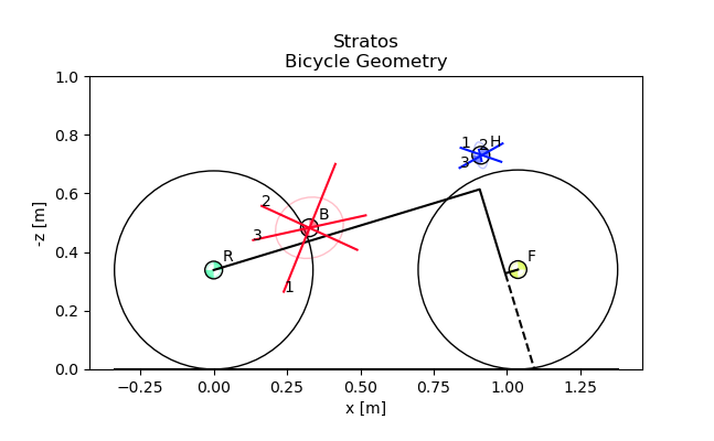
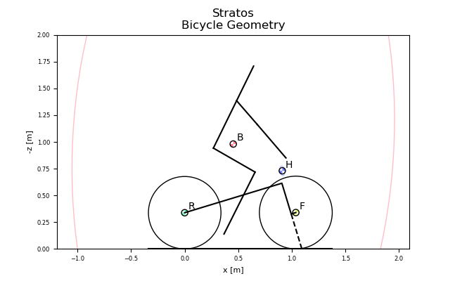
You can plot the geometry of the bicycle and include the mass centers of the various bodies, the inertia ellipsoids and the torsional pendulum axes from the raw measurement data:

_ = bicycle.plot_bicycle_geometry()

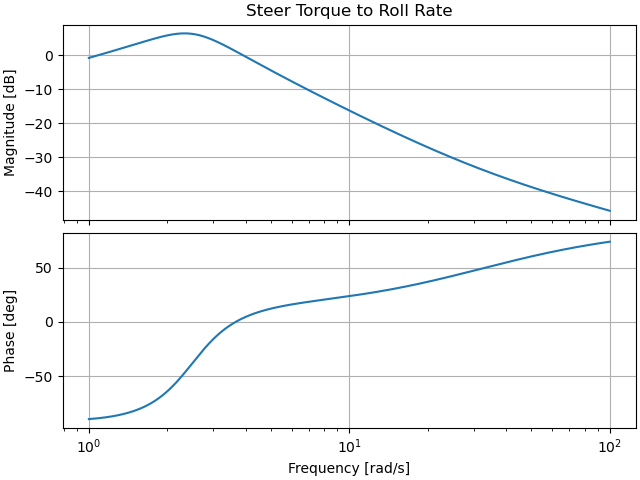
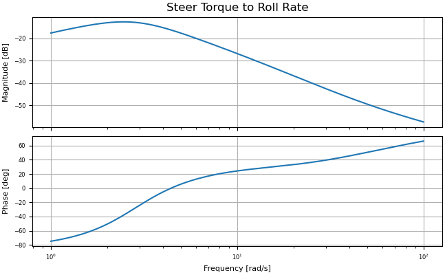
A Bode plot for any input output pair can be generated with:

_ = bicycle.plot_bode(3.0, 1, 2)

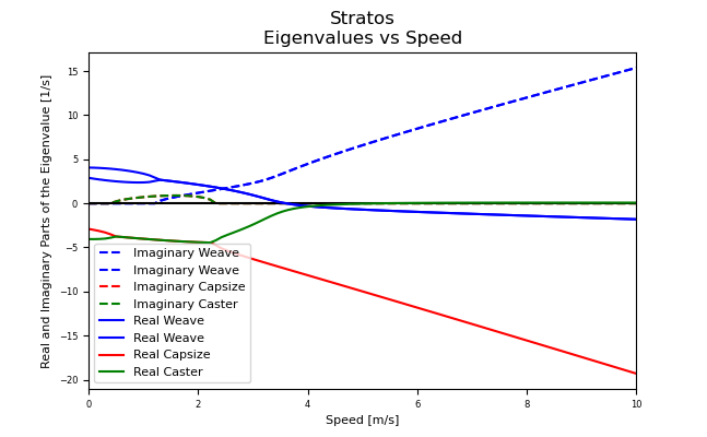
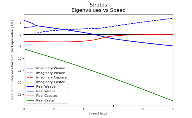
For visualization of the linear analysis you can plot the root loci of the real and imaginary parts of the eigenvalues as a function of speed:

speeds = np.linspace(0., 10., num=100)
_ = bicycle.plot_eigenvalues_vs_speed(speeds)

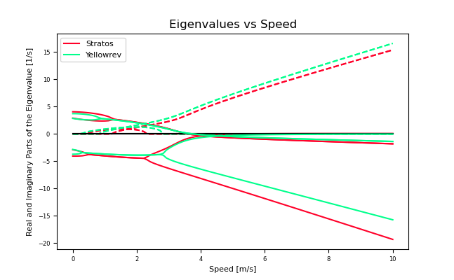
You can also compare the eigenvalues of two or more bicycles:

yellowrev = Bicycle('Yellowrev', pathToData='../data')
_ = bp.plot_eigenvalues([bicycle, yellowrev], speeds)

Found the RawData directory: ../data/bicycles/Yellowrev/RawData
Looks like you've already got some parameters for Yellowrev, use forceRawCalc to recalculate.

Tables

You can generate reStructuredText tables of the bicycle parameters with the Table class:

tab = tables.Table('Benchmark', False, (bicycle, yellowrev))
rst = tab.create_rst_table()
print(rst)

+----------+------------------+------------------+
|          | Stratos          | Yellowrev        |
+==========+=========+========+=========+========+
| Variable | v       | sigma  | v       | sigma  |
+----------+---------+--------+---------+--------+
| c        | 0.056   | 0.002  | 0.180   | 0.002  |
+----------+---------+--------+---------+--------+
| g        | 9.81    | 0.01   | 9.81    | 0.01   |
+----------+---------+--------+---------+--------+
| IBxx     | 0.373   | 0.002  | 0.2254  | 0.0009 |
+----------+---------+--------+---------+--------+
| IBxz     | -0.0383 | 0.0004 | 0.0179  | 0.0001 |
+----------+---------+--------+---------+--------+
| IByy     | 0.717   | 0.003  | 0.388   | 0.005  |
+----------+---------+--------+---------+--------+
| IBzz     | 0.455   | 0.002  | 0.2147  | 0.0009 |
+----------+---------+--------+---------+--------+
| IFxx     | 0.0916  | 0.0004 | 0.0852  | 0.0003 |
+----------+---------+--------+---------+--------+
| IFyy     | 0.157   | 0.001  | 0.147   | 0.002  |
+----------+---------+--------+---------+--------+
| IFzz     | 0.0916  | 0.0004 | NA      | NA     |
+----------+---------+--------+---------+--------+
| IHxx     | 0.1768  | 0.0008 | 0.1475  | 0.0006 |
+----------+---------+--------+---------+--------+
| IHxz     | -0.0273 | 0.0006 | -0.0172 | 0.0005 |
+----------+---------+--------+---------+--------+
| IHyy     | 0.144   | 0.002  | 0.120   | 0.002  |
+----------+---------+--------+---------+--------+
| IHzz     | 0.0446  | 0.0003 | 0.0294  | 0.0004 |
+----------+---------+--------+---------+--------+
| IRxx     | 0.0939  | 0.0004 | 0.0877  | 0.0004 |
+----------+---------+--------+---------+--------+
| IRyy     | 0.154   | 0.001  | 0.149   | 0.001  |
+----------+---------+--------+---------+--------+
| IRzz     | 0.0939  | 0.0004 | NA      | NA     |
+----------+---------+--------+---------+--------+
| lam      | 0.295   | 0.003  | 0.339   | 0.003  |
+----------+---------+--------+---------+--------+
| mB       | 7.22    | 0.02   | 3.31    | 0.02   |
+----------+---------+--------+---------+--------+
| mF       | 3.33    | 0.02   | 1.90    | 0.02   |
+----------+---------+--------+---------+--------+
| mH       | 3.04    | 0.02   | 2.45    | 0.02   |
+----------+---------+--------+---------+--------+
| mR       | 3.96    | 0.02   | 2.57    | 0.02   |
+----------+---------+--------+---------+--------+
| rF       | 0.3400  | 0.0001 | 0.3419  | 0.0001 |
+----------+---------+--------+---------+--------+
| rR       | 0.3385  | 0.0001 | 0.3414  | 0.0001 |
+----------+---------+--------+---------+--------+
| w        | 1.037   | 0.002  | 0.985   | 0.002  |
+----------+---------+--------+---------+--------+
| xB       | 0.326   | 0.003  | 0.412   | 0.004  |
+----------+---------+--------+---------+--------+
| xH       | 0.911   | 0.004  | 0.919   | 0.005  |
+----------+---------+--------+---------+--------+
| zB       | -0.483  | 0.003  | -0.618  | 0.004  |
+----------+---------+--------+---------+--------+
| zH       | -0.730  | 0.002  | -0.816  | 0.002  |
+----------+---------+--------+---------+--------+

Which renders in Sphinx like:

	Stratos		Yellowrev
Variable	v	sigma	v	sigma
IBxx	0.373	0.002	0.2254	0.0009
IBxz	-0.0383	0.0004	0.0179	0.0001
IByy	0.717	0.003	0.388	0.005
IBzz	0.455	0.002	0.2147	0.0009
IFxx	0.0916	0.0004	0.0852	0.0003
IFyy	0.157	0.001	0.147	0.002
IHxx	0.1768	0.0008	0.1475	0.0006
IHxz	-0.0273	0.0006	-0.0172	0.0005
IHyy	0.144	0.002	0.120	0.002
IHzz	0.0446	0.0003	0.0294	0.0004
IRxx	0.0939	0.0004	0.0877	0.0004
IRyy	0.154	0.001	0.149	0.001
c	0.056	0.002	0.180	0.002
g	9.81	0.01	9.81	0.01
lam	0.295	0.003	0.339	0.003
mB	7.22	0.02	3.31	0.02
mF	3.33	0.02	1.90	0.02
mH	3.04	0.02	2.45	0.02
mR	3.96	0.02	2.57	0.02
rF	0.3400	0.0001	0.3419	0.0001
rR	0.3385	0.0001	0.3414	0.0001
w	1.037	0.002	0.985	0.002
xB	0.326	0.003	0.412	0.004
xH	0.911	0.004	0.919	0.005
zB	-0.483	0.003	-0.618	0.004
zH	-0.730	0.002	-0.816	0.002

Adding a Rigid Rider

The program also allows one to add the inertial affects of a rigid rider to the Whipple bicycle model.

Rider Data

You can provide rider data in one of two ways, much in the same way as the bicycle. If you have the inertial parameters of a rider, e.g. Jason, simply add a file into the ./riders/Jason/Parameters/ directory. Or if you have raw measurements of the rider add the two files to ./riders/Jason/RawData/. The yeadon documentation explains how to collect the data for a rider.

Adding a Rider

To add a rider key in:

bicycle.add_rider('Jason')

There is no rider on the bicycle, now adding Jason.
No parameter files found, calculating the human configuration.
/home/docs/checkouts/readthedocs.org/user_builds/bicycleparameters/checkouts/stable/bicycleparameters/rider.py:338: RuntimeWarning: The iteration is not making good progress, as measured by the
 improvement from the last five Jacobian evaluations.
  solution = fsolve(zero, guess)
Joint angle A1A2extension = 0.0021339788477382124 pi-rad is out of range. Must be between -1.0 and 0.0 pi-rad.
Joint angle B1B2extension = 0.0021339788477382124 pi-rad is out of range. Must be between -1.0 and 0.0 pi-rad.

The program first looks for a parameter for for Jason sitting on the Stratos and if it can’t find one, it looks for the raw data for Jason and computes the inertial parameters. You can force calculation from raw data with:

bicycle.add_rider('Jason', reCalc=True)

Exploring the rider

The bicycle has a few new attributes now that it has a rider:

bicycle.hasRider

True

bicycle.riderName

'Jason'

inertial parmeters of the rider

pprint.pprint(bicycle.riderPar)

{'Benchmark': {'IBxx': np.float64(9.360297604528963),
               'IBxz': np.float64(0.01640061915204971),
               'IByy': np.float64(9.840351664496836),
               'IBzz': np.float64(2.5154561357221947),
               'mB': np.float64(83.50000000000001),
               'xB': np.float64(0.4642273125970131),
               'yB': np.float64(0.0),
               'zB': np.float64(-1.0232877173495207)}}

this is a yeadon.human object representing the Jason

bicycle.human

<yeadon.human.Human object at 0x71240435f620>

try:
    bicycle.human.print_properties()
except:
    pass

Mass (kg):

83.50000

COM in global frame from bottom center of pelvis (Ls0) (m):

[[ 0.     ]
 [-0.19658]
 [ 0.08129]]

Inertia tensor in global frame about human's COM (kg-m^2):

[[9.84035 0.      0.     ]
 [0.      9.3603  0.0164 ]
 [0.      0.0164  2.51546]]

The bicycle parameters now reflect that a rigid rider has been added to the bicycle frame:

bicycle.parameters['Benchmark']['mB']

90.72000000000001+/-0.02

At this point, the uncertainties don’t necessarily offer much information for any of the parameters that are functions of the rider, because we do not have a good idea of the uncertainty in the human inertia calculations in the Yeadon method.

Analysis

The same linear analysis can be performed now that a rider has been added, albeit the reported values and graphs will reflect the fact that the bicycle frame has the added inertial effects of the rider.

Plots

The bicycle geometry plot now reflects that there is a rider on the bicycle and displays a simplified depiction:

_ = bicycle.plot_bicycle_geometry()

The Bode plot reflects the changes:

_ = bicycle.plot_bode(3.0, 1, 2)

The eigenvalue plot reflects the changes:

_ = bicycle.plot_eigenvalues_vs_speed(speeds)