Example Usage
The Data
The program requires input data in the form of basic text files and a particular file system directory structure to organize the data. To use the program you will need to navigate to a directory where you have at least one directory named for a bicycle that contains parameters files or raw data measurements. Refer to the document BicycleParameters Data File Information for details about what the data files should contain.
Data Directory
You will need to setup a directory (a directory named data is used in the
following examples) somewhere for the data input and output files. The
structure of the directory should look like this:
/data
|
-->/bicycles
|  |
|  -->/Bicyclea
|  |  |
|  |  -->/Parameters
|  |  |
|  |  -->/Photos
|  |  |
|  |  -->/RawData
|  |
|  -->/Bicycleb
|     |
|     -->/Parameters
|     |
|     -->/Photos
|     |
|     -->/RawData
-->/riders
   |
   -->/Ridera
      |
      -->/Parameters
      |
      -->/RawData
Bicycle/rider name
A bicycle or rider name is a descriptive word (or compound word) for a bicycle or
rider in which the first letter is capitalized. Examples of bicycle short names
include Bianchipista, Bike, Mybike, Rigidrider,
Schwintandem, Gyrobike, Bicyclea, etc. Examples of rider names
include Jason, Mont, Lukepeterson, etc. The program relies on
CamelCase words, so make sure the first letter is capitalized and no others
are.
bicycles Directory
The bicycles directory contains subdirectories for each bicycle. The
directory name for a bicycle should be its bicycle name. Each directory in
bicycles should contain at least a RawData directory or a Parameters
directory. Photos is an optional directory.
RawData directory
You can supply raw measurement data in two forms:
A file containing all the manual measurements (including the oscillation periods for each rigid body). Refer to bicycles/<bicycle name>/RawData/<bicycle name>Measured.txt for details about the contents of this file.
A file containing all the manual measurements (not including the oscillation periods for each rigid body) and a set of data files containing oscillatory signals from which the periods can be estimated. Refer to Pendulum Data Files for details about these files.
The manual measurement data file should follow the naming convention <bicycle
name>Measure.txt. This data is used to generate parameter files that can be
saved to the Parameters directory.
Parameters directory
If you don’t have any raw measurements for the bicycle it is also an option to
supply a parameter file in the Parameters directory. Simply add a file named
<bicycle name>Benchmark.txt with the benchmark parameter set into the
Parameters directory for the particular bicycle. Refer to
bicycles/<bicycle name>/Parameters/<bicycle name>Benchmark.txt for details about the contents of the file.
Photos directory
The Photos folder should contain photos of the bicycle parts hung as the
various pendulums in the various orientations. The filename should follow the
conventions of the raw signal data files.
riders directory
The riders directory should contain a directory for each rider that you have
data for. The individual rider directory contains a Parameters for the
rider inertial parameters sets and a RawData directory for the raw
measurements needed for the Yeadon inertia model. Refer to riders/<rider name>/Parameters/
for details about these input files.
Example Data
Example data is available here:
Loading bicycle data
The easiest way to load a bicycle is:
>>> import bicycleparameters as bp
>>> bicycle = bp.Bicycle('Stratos')
This will create an instance of the Bicycle class in the variable bicycle based
off of input data from the ./bicycles/Stratos/ directory. The program first
looks to see if there are any parameter sets in
./bicycles/Stratos/Parameters/. If so, it loads the data, if not it looks
for ./bicycles/Stratos/RawData/StratosMeasurments.txt so that it can
generate the parameter set. The raw measurement file may or may not contain the
oscillation period data for the bicycle moment of inertia caluclations. If it
doesn’t then the program will look for the series of .mat files need to
calculate the periods. If no data is there, then you get an error.
There are other loading options:
>>> bicycle = bp.Bicycle('Stratos', pathToData='<some path to the data directory>', forceRawCalc=True, forcePeriodCalc=True)
The pathToData option allows you specify a directory other than the current
directory as your data directory. The forceRawCalc forces the program to
load ./bicycles/Stratos/RawData/StratosMeasurments.txt and recalculate the
parameters regarless if there are any parameter files available in
./bicycles/Stratos/Parameters/. The forcePeriodCalc option forces the period
calcluation from the .mat files regardless if they already exist in the raw
measurement file.
Exploring bicycle parameter data
The bicycle has a name:
>>> bicycle.bicycleName
'Stratos'
and a directory where its data is stored:
>>> bicycle.direcotory
'./bicycles/Stratos'
The benchmark bicycle parameters are the fundamental parameter set that is used behind the scenes for calculations. To access them type:
>>> bPar = bicycle.parameters['Benchmark']
>>> bPar['xB']
0.32631503794489763+/-0.0032538862692938642
The program automatically calculates the uncertainties in the parameters based on the raw measurements or the uncertainties provided in the parameter files. If you’d like to work with the pure values you can remove them:
>>> bParPure = bp.io.remove_uncertainties(bPar)
>>> bParPure['xB']
0.32631503794489763
That goes the same for all values with uncertainties. Check out the uncertainties package details for more ways to manipulate the quantities.
If the bicycle was calculated from raw data measurements you can access them by:
>>> bicycle.parameters['Measurements']
All parameter sets are stored in the parameter dictionary of the bicycle instance.
To modify a parameter type:
>>> bicycle.parameters['Benchmark']['mB'] = 50.
You can regenerate the parameter sets from the raw data stored in the bicycle’s directory by calling:
>>> bicycle.calculate_from_measured()
Basic Analysis
The program has some basic bicycle analysis tools based on the Whipple bicycle model which has been linearized about the upright configuration.
The canonical matrices for the equations of motion can be computed:
>>> M, C1, K0, K2 = bicycle.canonical()
>>> M
array([[4.87735569387+/-0.0239343413077, 0.407911475492+/-0.00852495589396],
      [0.407911475492+/-0.00852495589396,
       0.203245633856+/-0.00235820505536]], dtype=object)
>>> C1
array([[0.0, 4.85200252888+/-0.0242948940194],
      [-0.488808930325+/-0.00358710467251,
       0.751423298199+/-0.0118190412791]], dtype=object)
>>> K0
array([[-8.1786550655+/-0.0281976329402,
        -0.709791925937+/-0.013158888468],
       [-0.709791925937+/-0.013158888468,
        -0.206338069868+/-0.00571395841832]], dtype=object)
>>> K2
array([[0.0,
        8.39212115462+/-0.0313979563061],
       [0.0,
        0.778591689057+/-0.0128042478172]], dtype=object))
as well as the state and input matrices for state space form at a particular speed (1.34 m/s):
>>> A, B = bicycle.state_space(1.34)
>>> A
array([[0.0, 0.0, 1.0, 0.0],
       [0.0, 0.0, 0.0, 1.0],
       [16.324961319+/-0.039204516678, -2.30677907291+/-0.00824125009025,
        -0.323894489886+/-0.00578005141184,
        -1.10401174487+/-0.00684136323415],
       [1.49533216875+/-0.153839831788, 7.71036924174+/-0.170699435465,
        3.8727732103+/-0.0342265538607, -2.73840155487+/-0.0133666010323]], dtype=object)
>>> B
array([[0.0, 0.0],
       [0.0, 0.0],
       [0.246385378456+/-0.00169761878443,
        -0.494492409794+/-0.00770906162244],
       [-0.494492409794+/-0.00770906162244, 5.91259504914+/-0.0401866728435]], dtype=object)
You can calculate the eigenvalues and eigenvectors at any speed by calling:
>>> w, v = bicycle.eig(4.28) # the speed should be in meters/second
>>> w # eigenvalues
array([[-6.83490195+0.j        ,  0.46085314+2.77336727j,
         0.46085314-2.77336727j, -1.58257375+0.j        ]])
>>> v # eigenvectors
array([[[ 0.04283049+0.j        ,  0.50596715+0.33334818j,
          0.50596715-0.33334818j,  0.55478588+0.j        ],
        [ 0.98853840+0.j        ,  0.72150298+0.j        ,
          0.72150298+0.j        ,  0.63786241+0.j        ],
        [-0.00626644+0.j        ,  0.14646768-0.15809917j,
          0.14646768+0.15809917j, -0.35055926+0.j        ],
        [-0.14463096+0.j        ,  0.04206844-0.25316359j,
          0.04206844+0.25316359j, -0.40305383+0.j        ]]])
The eig function also accepts a one dimensional array of speeds and returns
eigenvalues for all speeds. Note that uncertainty propagation into the
eigenvalue calculations is not supported yet.
The moment of inertia of the steer assembly (handlebar, fork and/or front wheel) can be computed either about the center of mass or a point on the steer axis, both with reference to a frame aligned with the steer axis:
>>> bicycle.steer_assembly_moment_of_inertia(aboutSteerAxis=True)
array([[0.539931205836+/-0.00362870864185, 0.0,
        0.00921422347873+/-0.00191753741975],
       [0.0, 0.578940852064+/-0.00311525776442, 0.0],
       [0.00921422347873+/-0.00191753741975, 0.0,
        0.143206097868+/-0.00100279291208]], dtype=object)
Plots
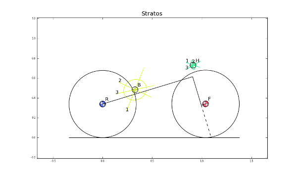
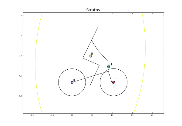
You can plot the geometry of the bicycle and include the mass centers of the various bodies, the inertia ellipsoids and the torsional pendulum axes from the raw measurement data:
>>> bicycle.plot_bicycle_geometry()
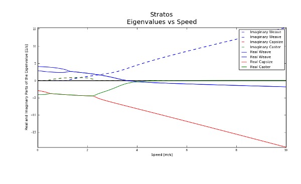
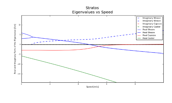
For visualization of the linear analysis you can plot the root loci of the real and imaginary parts of the eigenvalues as a function of speed:
>>> import numpy as np
>>> speeds = np.linspace(0., 10., num=100)
>>> bicycle.plot_eigenvalues_vs_speed(speeds, show=True)
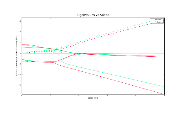
You can also compare the eigenvalues of two or more bicycles:
>>> yellowrev = bp.Bicycle('Yellowrev')
>>> bp.plot_eigenvalues([bicycle, yellowrev], speeds, show=True)
Tables
You can generate reStructuredText tables of the bicycle parameters with the
Table class:
>>> from bicycleparameters import tables
>>> tab = tables.Table('Measured', False, bicycle, yellowrev)
>>> rst = tab.create_rst_table()
>>> print rst
+----------+------------------+------------------+
|          | Stratos          | Yellowrev        |
+==========+=========+========+=========+========+
| Variable | v       | sigma  | v       | sigma  |
+----------+---------+--------+---------+--------+
| IBxx     | 0.373   | 0.002  | 0.2254  | 0.0009 |
+----------+---------+--------+---------+--------+
| IBxz     | -0.0383 | 0.0004 | 0.0179  | 0.0001 |
+----------+---------+--------+---------+--------+
| IByy     | 0.717   | 0.003  | 0.388   | 0.005  |
+----------+---------+--------+---------+--------+
| IBzz     | 0.455   | 0.002  | 0.2147  | 0.0009 |
+----------+---------+--------+---------+--------+
| IFxx     | 0.0916  | 0.0004 | 0.0852  | 0.0003 |
+----------+---------+--------+---------+--------+
| IFyy     | 0.157   | 0.001  | 0.147   | 0.002  |
+----------+---------+--------+---------+--------+
| IHxx     | 0.1768  | 0.0008 | 0.1475  | 0.0006 |
+----------+---------+--------+---------+--------+
| IHxz     | -0.0273 | 0.0006 | -0.0172 | 0.0005 |
+----------+---------+--------+---------+--------+
| IHyy     | 0.144   | 0.002  | 0.120   | 0.002  |
+----------+---------+--------+---------+--------+
| IHzz     | 0.0446  | 0.0003 | 0.0294  | 0.0004 |
+----------+---------+--------+---------+--------+
| IRxx     | 0.0939  | 0.0004 | 0.0877  | 0.0004 |
+----------+---------+--------+---------+--------+
| IRyy     | 0.154   | 0.001  | 0.149   | 0.001  |
+----------+---------+--------+---------+--------+
| c        | 0.056   | 0.002  | 0.180   | 0.002  |
+----------+---------+--------+---------+--------+
| g        | 9.81    | 0.01   | 9.81    | 0.01   |
+----------+---------+--------+---------+--------+
| lam      | 0.295   | 0.003  | 0.339   | 0.003  |
+----------+---------+--------+---------+--------+
| mB       | 7.22    | 0.02   | 3.31    | 0.02   |
+----------+---------+--------+---------+--------+
| mF       | 3.33    | 0.02   | 1.90    | 0.02   |
+----------+---------+--------+---------+--------+
| mH       | 3.04    | 0.02   | 2.45    | 0.02   |
+----------+---------+--------+---------+--------+
| mR       | 3.96    | 0.02   | 2.57    | 0.02   |
+----------+---------+--------+---------+--------+
| rF       | 0.3400  | 0.0001 | 0.3419  | 0.0001 |
+----------+---------+--------+---------+--------+
| rR       | 0.3385  | 0.0001 | 0.3414  | 0.0001 |
+----------+---------+--------+---------+--------+
| w        | 1.037   | 0.002  | 0.985   | 0.002  |
+----------+---------+--------+---------+--------+
| xB       | 0.326   | 0.003  | 0.412   | 0.004  |
+----------+---------+--------+---------+--------+
| xH       | 0.911   | 0.004  | 0.919   | 0.005  |
+----------+---------+--------+---------+--------+
| zB       | -0.483  | 0.003  | -0.618  | 0.004  |
+----------+---------+--------+---------+--------+
| zH       | -0.730  | 0.002  | -0.816  | 0.002  |
+----------+---------+--------+---------+--------+
Which renders in Sphinx like:
Stratos |
Yellowrev |
|||
|---|---|---|---|---|
Variable |
v |
sigma |
v |
sigma |
IBxx |
0.373 |
0.002 |
0.2254 |
0.0009 |
IBxz |
-0.0383 |
0.0004 |
0.0179 |
0.0001 |
IByy |
0.717 |
0.003 |
0.388 |
0.005 |
IBzz |
0.455 |
0.002 |
0.2147 |
0.0009 |
IFxx |
0.0916 |
0.0004 |
0.0852 |
0.0003 |
IFyy |
0.157 |
0.001 |
0.147 |
0.002 |
IHxx |
0.1768 |
0.0008 |
0.1475 |
0.0006 |
IHxz |
-0.0273 |
0.0006 |
-0.0172 |
0.0005 |
IHyy |
0.144 |
0.002 |
0.120 |
0.002 |
IHzz |
0.0446 |
0.0003 |
0.0294 |
0.0004 |
IRxx |
0.0939 |
0.0004 |
0.0877 |
0.0004 |
IRyy |
0.154 |
0.001 |
0.149 |
0.001 |
c |
0.056 |
0.002 |
0.180 |
0.002 |
g |
9.81 |
0.01 |
9.81 |
0.01 |
lam |
0.295 |
0.003 |
0.339 |
0.003 |
mB |
7.22 |
0.02 |
3.31 |
0.02 |
mF |
3.33 |
0.02 |
1.90 |
0.02 |
mH |
3.04 |
0.02 |
2.45 |
0.02 |
mR |
3.96 |
0.02 |
2.57 |
0.02 |
rF |
0.3400 |
0.0001 |
0.3419 |
0.0001 |
rR |
0.3385 |
0.0001 |
0.3414 |
0.0001 |
w |
1.037 |
0.002 |
0.985 |
0.002 |
xB |
0.326 |
0.003 |
0.412 |
0.004 |
xH |
0.911 |
0.004 |
0.919 |
0.005 |
zB |
-0.483 |
0.003 |
-0.618 |
0.004 |
zH |
-0.730 |
0.002 |
-0.816 |
0.002 |
Rigid Rider
The program also allows one to add the inertial affects of a rigid rider to the Whipple bicycle system.
Rider Data
You can provide rider data in one of two ways, much in the same way as the
bicycle. If you have the inertial parameters of a rider, e.g. Jason, simply add
a file into the ./riders/Jason/Parameters/ directory. Or if you have raw
measurements of the rider add the two files to ./riders/Jason/RawData/. The
yeadon documentation explains how to collect the data for a rider.
Adding a Rider
To add a rider key in:
>>> bicycle.add_rider('Jason')
The program first looks for a parameter for for Jason sitting on the Stratos and if it can’t find one, it looks for the raw data for Jason and computes the inertial parameters. You can force calculation from raw data with:
>>> bicycle.add_rider('Jason', reCalc=True)
Exploring the rider
The bicycle has a few new attributes now that it has a rider:
>>> bicycle.hasRider
True
>>> bicycle.riderName
'Jason'
>>> bicycle.riderPar # inertial parmeters of the rider
{'Benchmark': {'IBxx': 7.8188533619237681,
               'IBxz': -0.035425693766513083,
               'IByy': 8.2729669089020437,
               'IBzz': 2.354736583109867,
               'mB': 79.152920866435153,
               'xB': 0.46614935153554904,
               'yB': 2.1457815736317352e-07,
               'zB': -1.0385521459829261}}
>>> bicycle.human # this is a yeadon.human object representing the Jason
<yeadon.human.human instance at 0x2b19dd0>
The bicycle parameters now reflect that a rigid rider has been added to the bicycle frame:
>>> bicycle.parameters['Benchmark']['mB']
86.37292086643515+/-0.02
At this point, the uncertainties don’t necessarily offer much information for any of the parameters that are functions of the rider, because we do not have a good idea of the uncertainty in the human inertia calculations in the Yeadon method.
Analysis
The same linear analysis can be performed now that a rider has been added, albeit the reported values and graphs will reflect the fact that the bicycle frame has the added inertial effects of the rider.
Plots
The bicycle geometry plot now reflects that there is a rider on the bicycle and displays a simplified depiction:
>>> bicycle.plot_bicycle_geometry()
The eigenvalue plot also relfects the changes:
>>> bicycle.plot_eigenvalues_vs_speed(speeds, show=True)
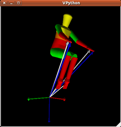
Rider Visualization
If you have the optional dependency, visual python, for yeadon installed then you can output a three dimensional picture of the Yeadon model configured to be seated on the bicycle. This is a bit buggy due to the nature of visual python, but is useful none-the-less.:
>>> bicycle.add_rider('Jason', draw=True)
Using Models and Parameter Sets
Parameter Sets
Parameter sets represent a set of constants in a multibody dynamics model.
These constants have a name and an associated floating point value. This
mapping from name to value is stored in a dictionary and then passed to a
ParameterSet. Below are the parameters for the Meijaard et al. 2007
paper with some realistic initial values.
par = {
    'IBxx': 11.3557360401,
    'IBxz': -1.96756380745,
    'IByy': 12.2177848012,
    'IBzz': 3.12354397008,
    'IFxx': 0.0904106601579,
    'IFyy': 0.149389340425,
    'IHxx': 0.253379594731,
    'IHxz': -0.0720452391817,
    'IHyy': 0.246138810935,
    'IHzz': 0.0955770796289,
    'IRxx': 0.0883819364527,
    'IRyy': 0.152467620286,
    'c': 0.0685808540382,
    'g': 9.81,
    'lam': 0.399680398707,
    'mB': 81.86,
    'mF': 2.02,
    'mH': 3.22,
    'mR': 3.11,
    'rF': 0.34352982332,
    'rR': 0.340958858855,
    'v': 1.0,
    'w': 1.121,
    'xB': 0.289099434117,
    'xH': 0.866949640247,
    'zB': -1.04029228321,
    'zH': -0.748236400835,
}
The associated parameter set can be created with this dictionary:
from bicycleparameters.parameter_sets import Meijaard2007ParameterSet

par_set = Meijaard2007ParameterSet(par, True)
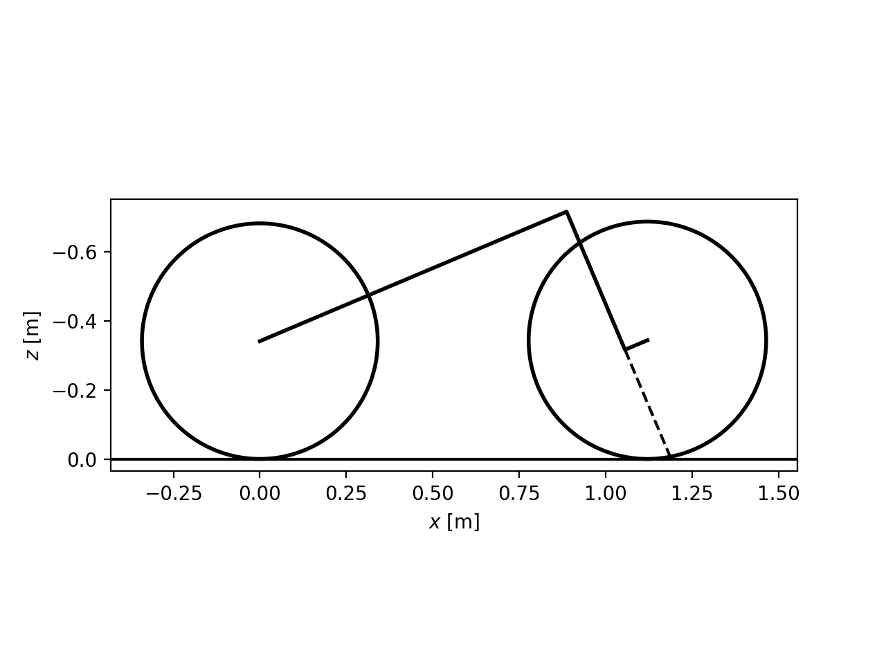
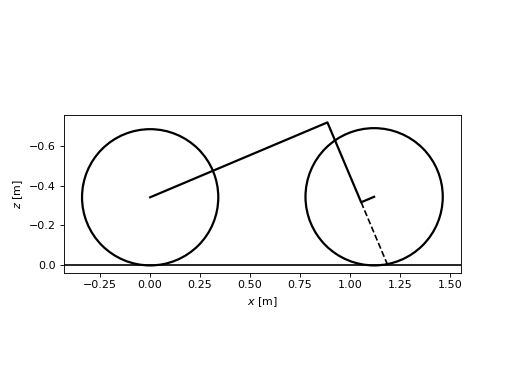
Once the parameter set is available there are various methods that help you calculate and visualize the properties of this parameter set. This set describes the geometry, mass, and inertia of a bicycle. You can plot the geometry like so:
par_set.plot_geometry()
(Source code, png, hires.png, pdf)
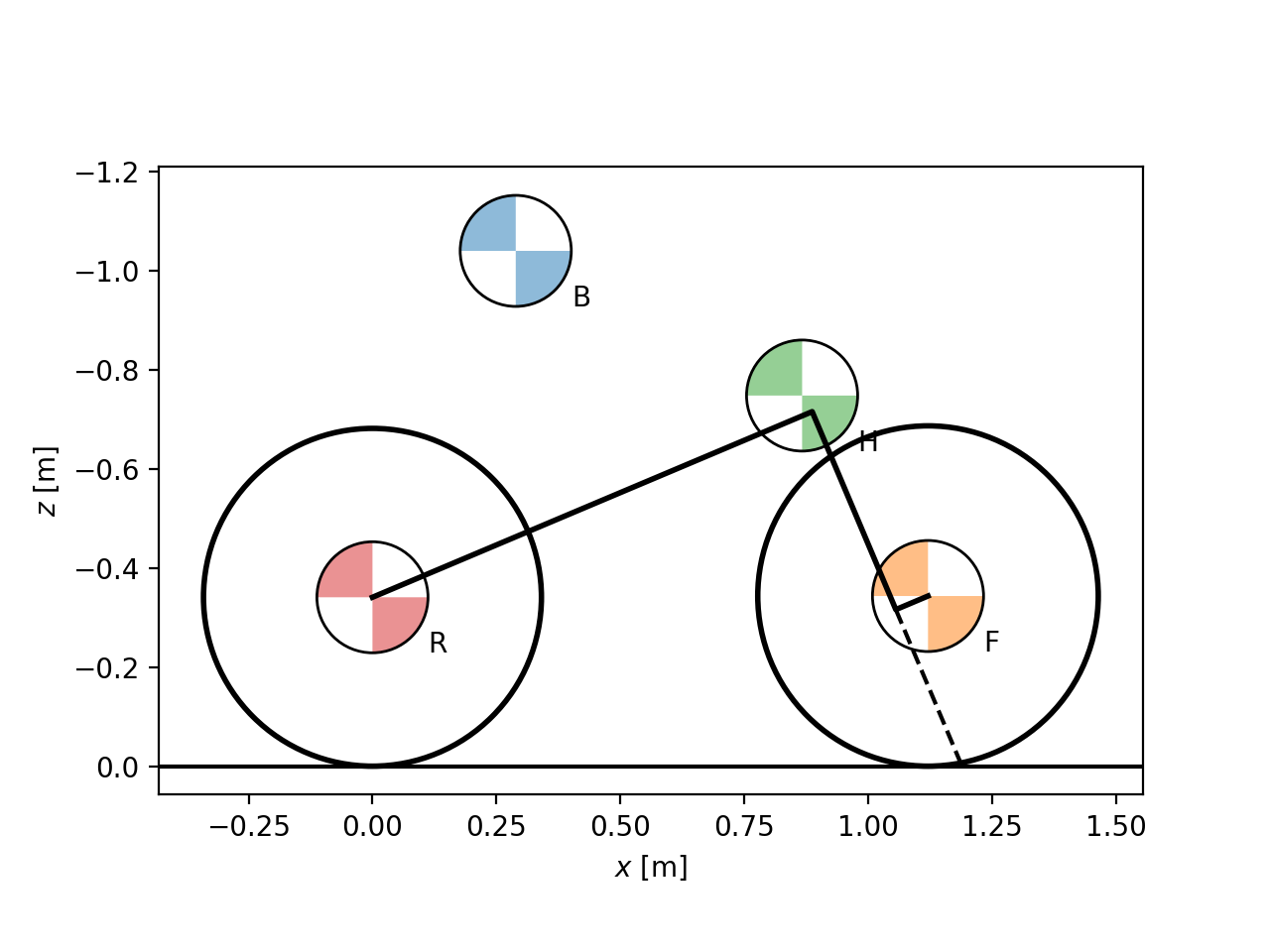
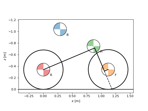
You can then add symbols representing the mass centers of the four bodies like so:
ax = par_set.plot_geometry()
par_set.plot_mass_centers(ax=ax)
(Source code, png, hires.png, pdf)
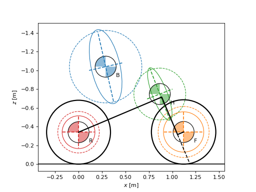
The geometry, mass, and inertial information can all be plotted:
par_set.plot_all()
(Source code, png, hires.png, pdf)

Models
Parameter sets can be associated with a model and the model can be used to compute and visualize properties of the model’s dynamics.
from bicycleparameters.models import Meijaard2007Model

model = Meijaard2007Model(par_set)
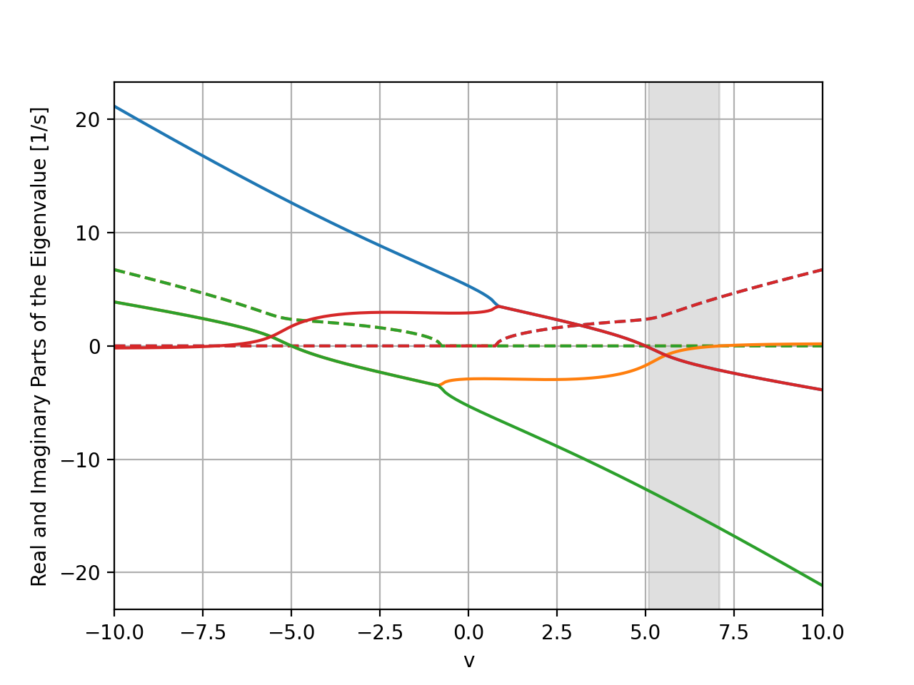
The root locus with respect to any parameter, for example speed v, can be
plotted:
speeds = np.linspace(-10.0, 10.0, num=200)

model.plot_eigenvalue_parts(v=speeds)
(Source code, png, hires.png, pdf)

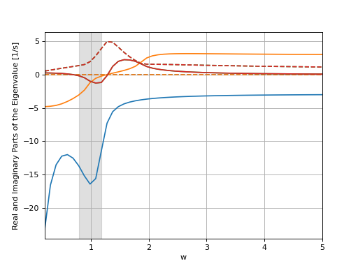
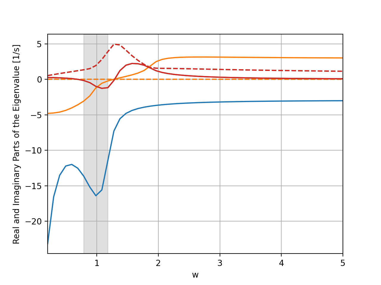
You can choose any parameter in the dictionary to generate the root locus and also override other parameters.
wheelbases = np.linspace(0.2, 5.0, num=50)

model.plot_eigenvalue_parts(v=6.0, w=wheelbases)
(Source code, png, hires.png, pdf)

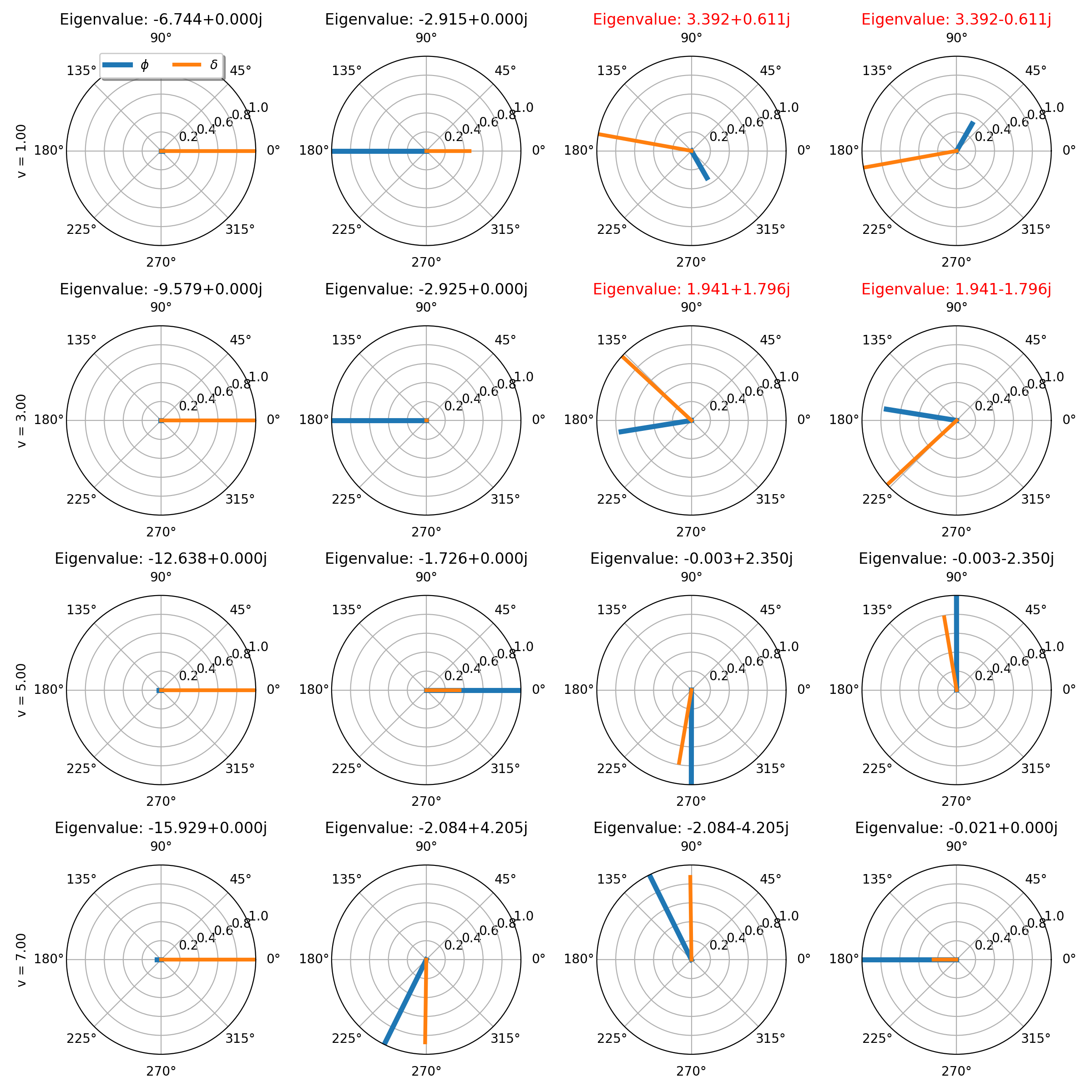
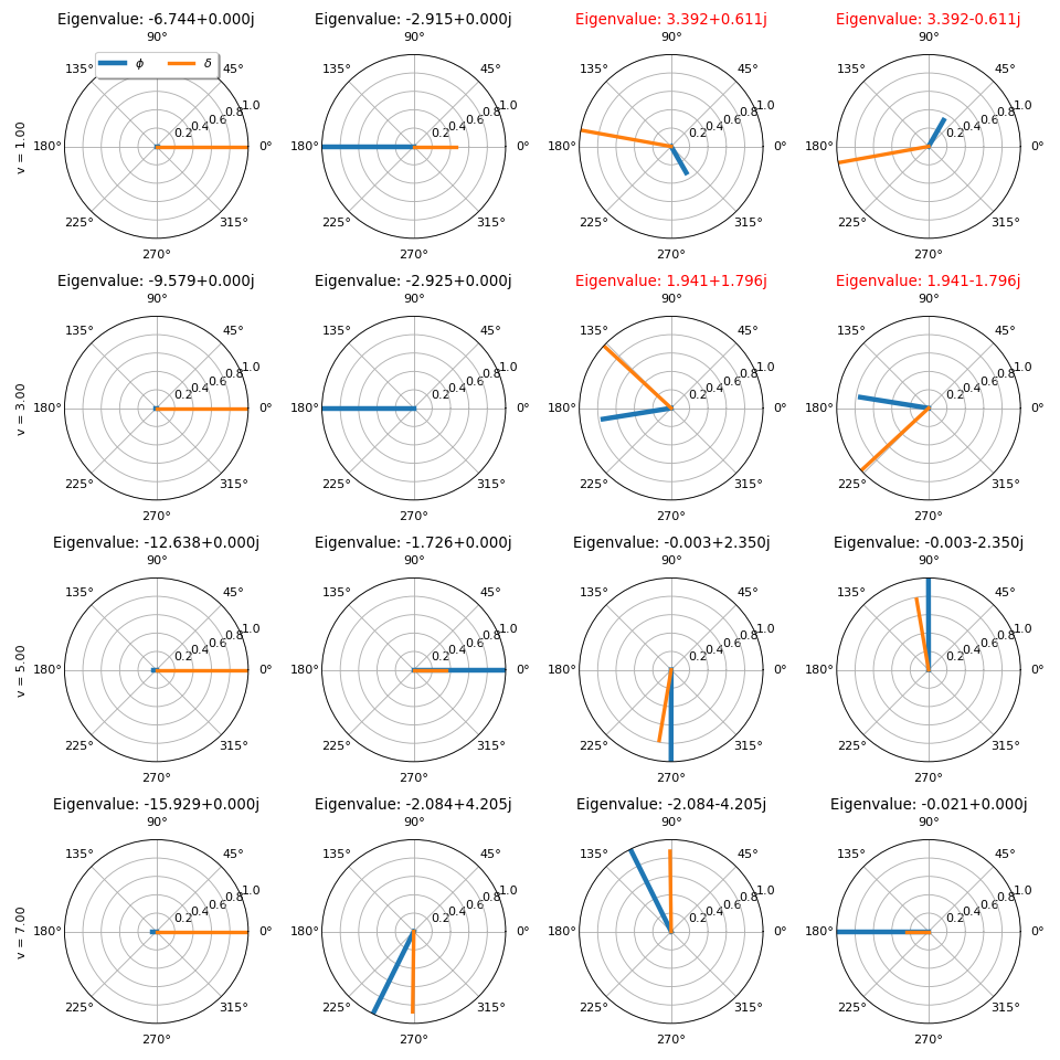
The eigenvector components can be created for each mode and for a series of parameter values:
model.plot_eigenvectors(v=[1.0, 3.0, 5.0, 7.0])
(Source code, png, hires.png, pdf)
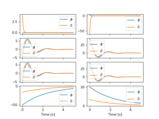
The eigenmodes can be simulated for specific parameter values:
times = np.linspace(0.0, 5.0, num=100)

model.plot_mode_simulations(times, v=6.0)
(Source code, png, hires.png, pdf)

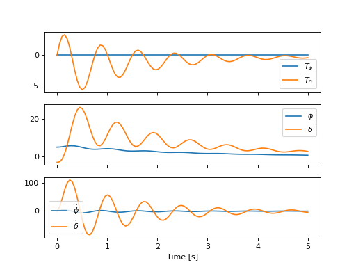
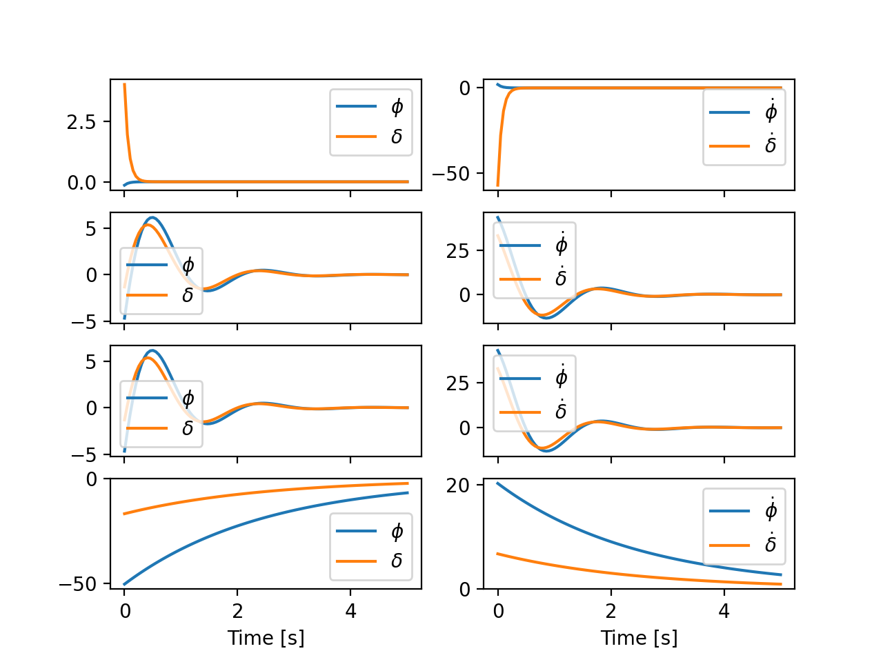
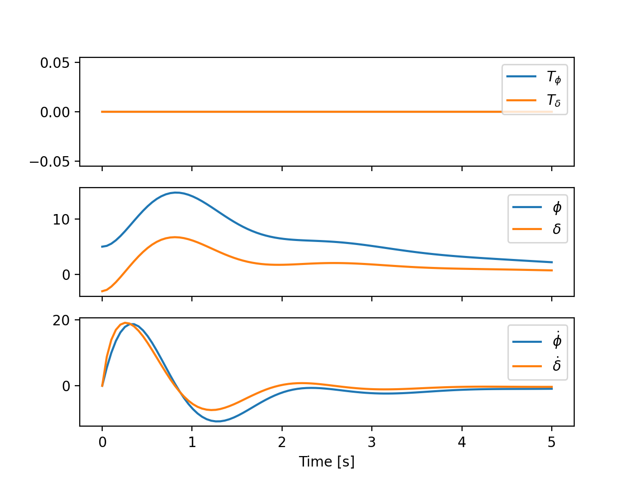
A general simulation from initial conditions can also be run:
x0 = np.deg2rad([5.0, -3.0, 0.0, 0.0])

model.plot_simulation(times, x0, v=6.0)
(Source code, png, hires.png, pdf)

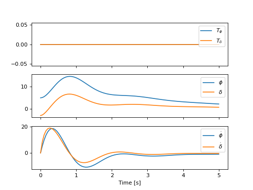
Inputs can be applied in the simulation, for example a simple positive feedback derivative controller on roll:
x0 = np.deg2rad([5.0, -3.0, 0.0, 0.0])

model.plot_simulation(times, x0,
    input_func=lambda t, x: np.array([0.0, 50.0*x[2]]),
    v=2.0)
(Source code, png, hires.png, pdf)